物理信息学习

由于 TensorMesh 的每个算子都被 autograd 追踪,装配好的 FEM 系统本身就可以充当训练神经网络的损失。我们不是去 求解 K u = F,而是用一个网络 \(u_\theta(x, y)\) 表示解,并最小化弱形式的 离散伽辽金残差:
其中 \(u_\theta\) 是在网格节点处求值的网络。该残差是由 TensorMesh 装配的 FEM(弱形式)残差——而非强形式配点残差——并且由于 SparseMatrix.__matmul__ 是可微的,loss = ||K u_theta - F||^2 会直接反向传播到网络权重中。无需线性求解,无需手写伴随。
本示例库从单个泊松方程示例开始;该模式可推广到 TensorMesh 能够装配的任意弱形式。
通过伽辽金残差求解泊松方程 —— poisson_galerkin.py
求解
采用制造解 \(u = \sin\pi x\,\sin\pi y\)(因此 \(f = 2\pi^2\,\sin\pi x\,\sin\pi y\)),这使我们能够将网络与解析场进行对照评分。
TensorMesh 一次性装配拉普拉斯刚度 \(K\) 和一致载荷 \(F = M f\);Condenser 将它们约化为内部系统 \(K_- u = F_-\)(齐次狄利克雷数据)。\(\|K_- u - F_-\|^2\) 的最小化解恰好是 FEM 解 \(K_-^{-1}F_-\),因此训练网络去复现它:
import torch
from tensormesh import (Mesh, LaplaceElementAssembler,
                        MassElementAssembler, Condenser)

class MLP(torch.nn.Module):              # (x, y) -> u
    def __init__(self, width=64, depth=3):
        super().__init__()
        layers = [torch.nn.Linear(2, width), torch.nn.Tanh()]
        for _ in range(depth - 1):
            layers += [torch.nn.Linear(width, width), torch.nn.Tanh()]
        layers += [torch.nn.Linear(width, 1)]
        self.net = torch.nn.Sequential(*layers)
    def forward(self, xy):
        return self.net(xy).squeeze(-1)

mesh = Mesh.gen_rectangle(chara_length=0.05)
K = LaplaceElementAssembler.from_mesh(mesh)().double()
M = MassElementAssembler.from_mesh(mesh)().double()
F = M @ f_nodal                                  # consistent load
K_, F_ = Condenser(mesh.boundary_mask)(K, F)     # interior system
coords = mesh.points[~mesh.boundary_mask]        # interior node coords

net = MLP().double()
opt = torch.optim.Adam(net.parameters(), lr=1e-3)
for step in range(8000):
    opt.zero_grad()
    u_theta = net(coords)
    loss = ((K_ @ u_theta - F_) ** 2).sum() / (F_ ** 2).sum()  # Galerkin residual
    loss.backward()                              # autograd through K_ @ u
    opt.step()
平方残差是病态的(其海森矩阵为 \(K_-^{T}K_-\)),因此——正如物理信息训练中的标准做法——在 Adam 预热之后接一段简短的 LBFGS 精修,将残差再压低一个数量级。
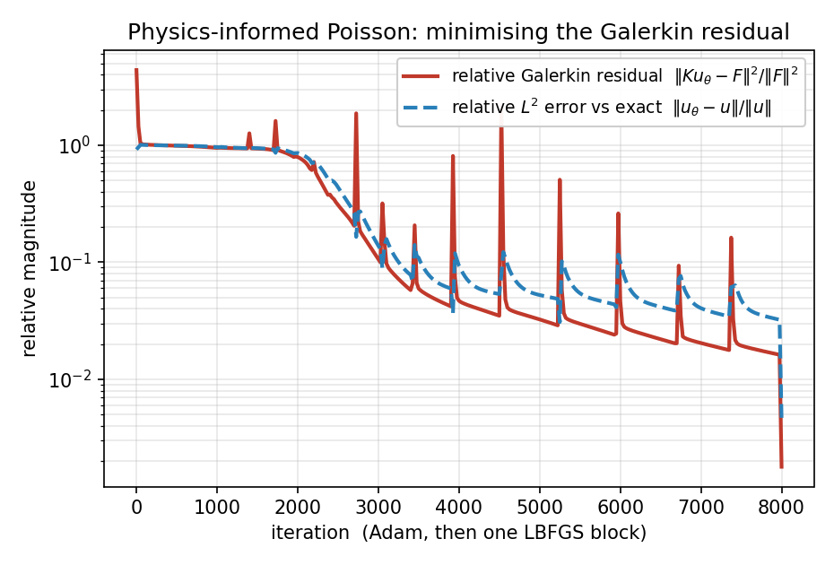
图 77 训练历史。相对伽辽金残差与相对于精确解的相对 \(L^2\) 误差都从 \(\mathcal{O}(1)\) 开始下降;周期性的尖峰是 Adam 过冲所致,而第 8000 次迭代处那一急剧的最终下降则来自 LBFGS 阶段。
学习到的场与解析解难以区分:
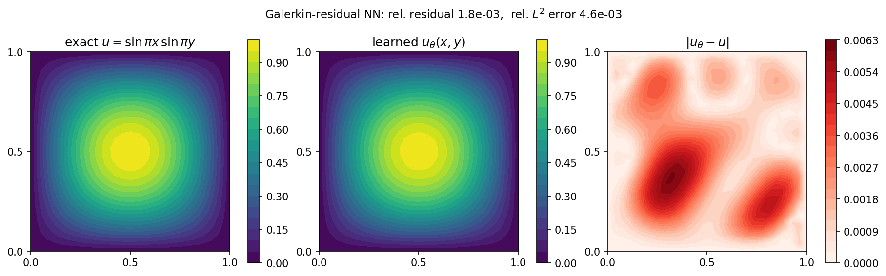
图 78 精确解 \(u\)(左)、学习到的 \(u_\theta\)(中),以及绝对误差(右,\(\le 6\times10^{-3}\))。网络相对于精确解的相对 \(L^2\) 误差约为 \(0.5\%\),相对于直接 FEM 求解的误差约为 \(0.3\%\)——也就是说,它在网格自身的离散化误差范围内复现了 FEM 解,在 CPU 上约耗时十秒。
备注
这是物理信息学习的 变分 / 伽辽金 类型:损失是装配好的弱形式残差,因此物理以与 FEM 中完全相同的方式进入(一次装配,每次迭代复用),而边界条件由 Condenser 处理,而非通过惩罚项。这里的网络是一个普通的 torch.nn.Module;将网络接入 TensorMesh 流水线的三种方式参见 可微性。
运行示例
cd examples/physics_informed
python poisson_galerkin.py        # ~10 s CPU -> poisson_galerkin_*.png
参数:--device cuda、--chara-length、--adam-iters、--lbfgs-iters、--width、--depth(-h 可查看列表)。