Physics-Informed Learning

Because every TensorMesh operator is autograd-traced, the assembled FEM system itself can serve as the loss for training a neural network. Rather than solving K u = F, we represent the solution by a network \(u_\theta(x, y)\) and minimise the discrete Galerkin residual of the weak form:

\[\min_{\theta}\;\; \big\| K\, u_\theta - F \big\|^2 ,\]

where \(u_\theta\) is the network evaluated at the mesh nodes. The residual is the FEM (weak-form) residual assembled by TensorMesh — not a strong-form collocation residual — and since SparseMatrix.__matmul__ is differentiable, loss = ||K u_theta - F||^2 back-propagates straight into the network weights. No linear solve, no hand-coded adjoint.

This gallery starts with a single Poisson example; the pattern extends to any weak form TensorMesh can assemble.

Poisson via the Galerkin residual — poisson_galerkin.py

Solve

\[-\Delta u = f \quad\text{in }(0,1)^2,\qquad u = 0 \text{ on }\partial\Omega,\]

with the manufactured solution \(u = \sin\pi x\,\sin\pi y\) (so \(f = 2\pi^2\,\sin\pi x\,\sin\pi y\)), which lets us score the network against an analytical field.

TensorMesh assembles the Laplace stiffness \(K\) and the consistent load \(F = M f\) once; Condenser reduces them to the interior system \(K_- u = F_-\) (homogeneous Dirichlet data). The minimiser of \(\|K_- u - F_-\|^2\) is exactly the FEM solution \(K_-^{-1}F_-\), so the network is trained to reproduce it:

import torch
from tensormesh import (Mesh, LaplaceElementAssembler,
                        MassElementAssembler, Condenser)

class MLP(torch.nn.Module):              # (x, y) -> u
    def __init__(self, width=64, depth=3):
        super().__init__()
        layers = [torch.nn.Linear(2, width), torch.nn.Tanh()]
        for _ in range(depth - 1):
            layers += [torch.nn.Linear(width, width), torch.nn.Tanh()]
        layers += [torch.nn.Linear(width, 1)]
        self.net = torch.nn.Sequential(*layers)
    def forward(self, xy):
        return self.net(xy).squeeze(-1)

mesh = Mesh.gen_rectangle(chara_length=0.05)
K = LaplaceElementAssembler.from_mesh(mesh)().double()
M = MassElementAssembler.from_mesh(mesh)().double()
F = M @ f_nodal                                  # consistent load
K_, F_ = Condenser(mesh.boundary_mask)(K, F)     # interior system
coords = mesh.points[~mesh.boundary_mask]        # interior node coords

net = MLP().double()
opt = torch.optim.Adam(net.parameters(), lr=1e-3)
for step in range(8000):
    opt.zero_grad()
    u_theta = net(coords)
    loss = ((K_ @ u_theta - F_) ** 2).sum() / (F_ ** 2).sum()  # Galerkin residual
    loss.backward()                              # autograd through K_ @ u
    opt.step()

The squared residual is ill-conditioned (its Hessian is \(K_-^{T}K_-\)), so — as is standard for physics-informed training — an Adam warm-up is followed by a short LBFGS refine, which drives the residual down by another order of magnitude.

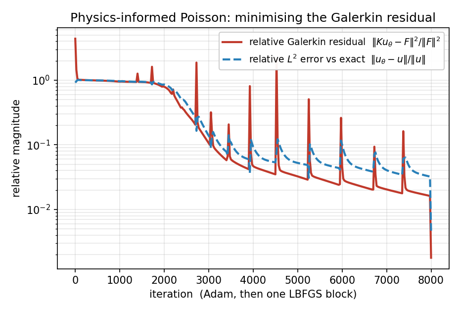
Fig. 55 Training history. Both the relative Galerkin residual and the relative \(L^2\) error against the exact solution fall from \(\mathcal{O}(1)\); the periodic spikes are Adam overshooting, and the sharp final drop at iteration 8000 is the LBFGS block.

The learned field is indistinguishable from the analytical solution:

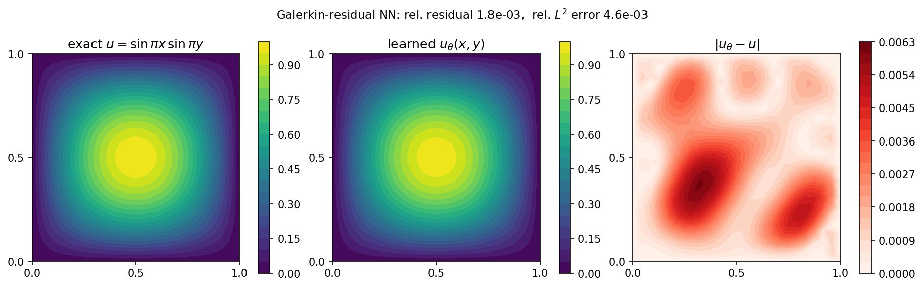
Fig. 56 Exact \(u\) (left), the learned \(u_\theta\) (middle), and the absolute error (right, \(\le 6\times10^{-3}\)). The network reaches a relative \(L^2\) error of about \(0.5\%\) against the exact solution and \(0.3\%\) against the direct FEM solve — i.e. it recovers the FEM solution to within the mesh’s own discretisation error, in about ten seconds on CPU.

Note

This is the variational / Galerkin flavour of physics-informed learning: the loss is the assembled weak-form residual, so the physics enters exactly as it does in the FEM (one assembly, reused every iteration) and boundary conditions are handled by Condenser rather than by a penalty term. The network here is a plain torch.nn.Module; see Differentiability for the three ways to wire a network into a TensorMesh pipeline.

Running the example

cd examples/physics_informed
python poisson_galerkin.py        # ~10 s CPU -> poisson_galerkin_*.png

Flags: --device cuda, --chara-length, --adam-iters, --lbfgs-iters, --width, --depth (-h for the list).

What’s next

• Differentiability — why the assembled system is differentiable and how gradients flow through SparseMatrix.

• Inverse Design & Identification — the same autograd machinery used for identification and design rather than for the forward solution.

• Poisson Equation — the classical (solved, not learned) Poisson examples.