Poisson Equation

Three scripts in examples/poisson/ walk the Poisson problem through TensorMesh’s main features: a basic 2D solve, the same solver in 3D, and h-adaptive refinement on an L-shaped domain whose re-entrant corner produces a gradient singularity.

For batched right-hand sides over many source terms (the ML data- generation pattern), see ML Datasets — that script lives under examples/dataset/poisson/ so all batched-RHS workflows sit in one place.

The strong form is:

\[-\Delta u = f \quad \text{in } \Omega, \qquad u = 0 \text{ on } \partial\Omega,\]

with corresponding weak form

\[\int_\Omega \nabla u \cdot \nabla v \,\mathrm{d}\Omega \;=\; \int_\Omega f\, v \,\mathrm{d}\Omega \quad \forall v \in H^1_0(\Omega).\]

Every example below realizes this with LaplaceElementAssembler for the stiffness, a NodeAssembler for the load, and Condenser for the homogeneous Dirichlet BC. The ground-truth source field comes from PoissonMultiFrequency, which generates a random truncated Fourier series whose analytical solution is also available.

Basic 2D Poisson — poisson.py

The shortest end-to-end driver in the repo. The full pipeline fits in 25 lines:

Listing 3 examples/poisson/poisson.py

import torch
from tensormesh import (LaplaceElementAssembler, Mesh,
                        Condenser, NodeAssembler)
from tensormesh.dataset import PoissonMultiFrequency

device         = "cuda" if torch.cuda.is_available() else "cpu"
mesh           = Mesh.gen_rectangle(chara_length=0.02).to(device=device)
assembler      = LaplaceElementAssembler.from_mesh(mesh)
equation       = PoissonMultiFrequency(K=16)
boundary_value = torch.zeros(mesh.boundary_mask.shape).to(device=device)
condenser      = Condenser(mesh.boundary_mask, boundary_value)

f = equation.source_term(mesh.points, domain="rectangle")
K = assembler(mesh.points)

class FAssembler(NodeAssembler):
    def forward(self, v, f):
        return v * f

F_asm = FAssembler.from_mesh(mesh)
b     = F_asm(mesh.points, point_data={"f": f})

K_, b_       = condenser(K, b)
u_           = K_.solve(b_, verbose=True)
u            = condenser.recover(u_)
u_analytical = equation.solution(mesh.points)

mesh.plot({"f": f, "u_fem": u, "u_analytical": u_analytical},
          save_path="poisson.png")

A few details worth pointing out:

• assembler(mesh.points) returns a SparseMatrix built from the gradient bilinear form. Pure-Python weak form, no custom kernels.

• FAssembler carries the source f through the integrand by name (point_data={"f": f} becomes the f kwarg in forward(v, f)). See Forms for the full argument-dispatch contract.

• The Condenser shorthand K_, b_ = condenser(K, b) applies the Dirichlet boundary mask and folds prescribed values into the RHS. recover(...) glues the boundary values back on after the solve.

• K_.solve(b_) is inherited from torch-sla’s SparseTensor; it inspects the matrix and dispatches to the best available backend automatically. Passing verbose=True prints that decision, e.g.:

  [torch-sla] solve: n=2814, nnz=19300, dtype=float64, device=cuda,
              symmetric=True, spd=False, backend=cudss, method=ldlt
  

  Here torch-sla detected a symmetric (but not SPD) system on CUDA and routed it through cuDSS with an \(LDL^{T}\) factorization. On CPU, or without cuDSS installed, it falls back to a different backend; the backend= field always tells you which one ran.

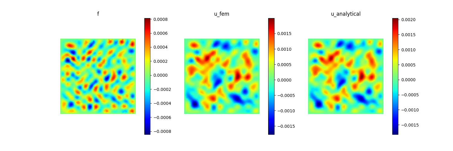
Fig. 38 Output of poisson.py: source f (left), FEM solution u_fem (middle), and analytical reference u_analytical (right) on the unit square. The two solution panels are visually indistinguishable at this resolution — exactly what you want from a converged mesh.

3D extension — poisson_3d.py

Identical machinery, swapping in a tetrahedral cube:

mesh = Mesh.gen_cube(chara_length=0.05, element_type="tet")
K    = LaplaceElementAssembler.from_mesh(mesh)()

The same LaplaceElementAssembler works because ∇u·∇v is dimension-generic — the integrand has no hard-coded spatial dimension. The output is written as poisson_3d.vtu for opening in ParaView; the script also produces a half-domain cutaway PNG for quick inspection.

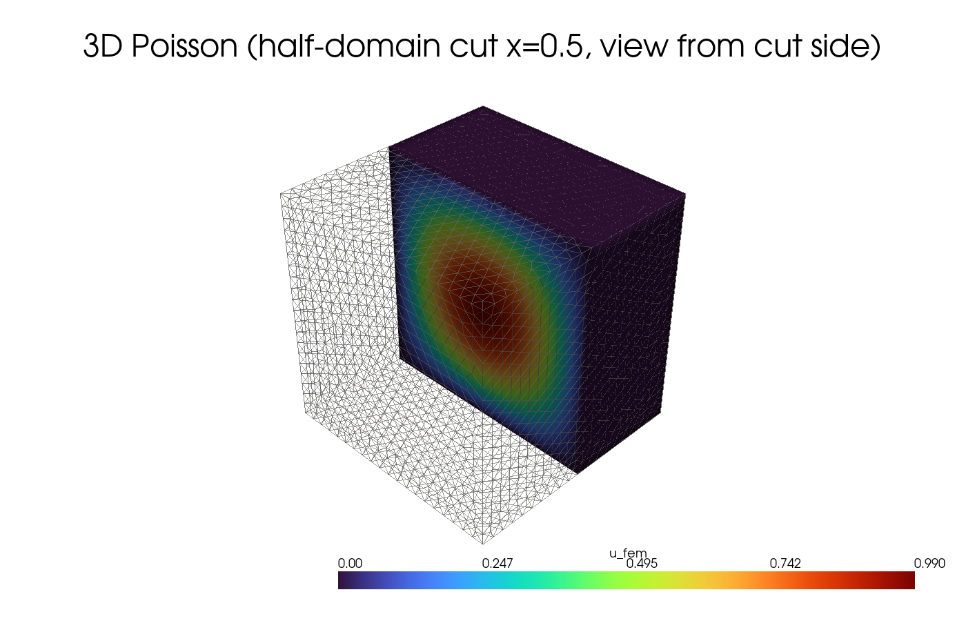
Fig. 39 Output of poisson_3d.py: half-domain cut at \(x=0.5\) showing the FEM solution on the unit cube. The reported mass-weighted relative \(L^2\) error against the analytical Fourier solution is \(\mathrm{rel\_L2} = 1.059\times10^{-2}\) at chara_length=0.05.

h-adaptive refinement on the L-shape — poisson_h_adaptivity.py

This is the one example on this page that goes well beyond the weak form. The L-shaped domain has a re-entrant corner at \((0.5, 0.5)\), where the exact solution \(u = r^{2/3}\sin(2\theta/3)\) has a gradient singularity. Uniform h-refinement converges slowly because the global error is dominated by the corner singularity.

The script implements the classical solve -> estimate -> mark -> remesh loop. For P1 triangles, u_fem is affine on each element, so \(\Delta u_h = 0\) inside every element for this Laplace problem. The residual estimator therefore comes from jumps of the normal gradient across interior edges:

\[\eta_K^2 = \sum_{e \subset \partial K \cap \Omega} h_e \left\| \left[\!\left[ \nabla u_h \cdot n_e \right]\!\right] \right\|^2_{L^2(e)}.\]

On a straight P1 edge the jump is constant, and the implementation uses the equivalent form \(\sum_e |e|^2 [[\nabla u_h \cdot n_e]]^2\). TensorMesh supplies the element gradients via Transformation and the interior-neighbor pairs via mesh.element_adjacency("triangle").

Listing 4 examples/poisson/poisson_h_adaptivity.py (essence)

mesh = Mesh.gen_L(chara_length=0.08, element_type="tri")
for level in range(max_levels):
    u_fem   = solve_laplace(mesh)
    u_exact = singular_solution(mesh.points)
    rel_err = global_l2_error(mesh, u_fem, u_exact)
    if rel_err < target_error:
        break
    centroids, eta, h = element_error_and_sizes(mesh, u_fem)
    h_new = doerfler_sizes(h, eta, theta=0.5)         # halve where eta > theta*max(eta)
    mesh  = remesh_L(centroids, h_new)                # gmsh remesh

Three pieces are worth a closer look:

• Non-homogeneous Dirichlet BC. The exact solution is non-zero on the boundary, so the script builds a Condenser with dirichlet_value=g evaluated from the singular formula at every boundary node. Static condensation folds the boundary values into the RHS; see Boundary Conditions.

• Mass-weighted reporting error. MassElementAssembler provides the \(L^2\) norm operator: e^T M e. The relative error divides by \(\sqrt{u_\text{exact}^T M u_\text{exact}}\) for scale invariance. This diagnostic uses the manufactured singular solution only to measure convergence; it does not drive refinement.

• Dörfler marking. Mark every element whose error indicator exceeds \(\theta\, \max(\eta)\) (default \(\theta=0.5\)) and halve its size; coarsen the (almost-)error-free elements. The new size field is fed to gmsh.model.mesh.setSizeCallback, and the L-shape geometry is re-meshed via OpenCASCADE booleans.

Note

The remesh step calls into gmsh directly via the Python API and requires gmsh >= 4.8 for setSizeCallback. Install with pip install gmsh.

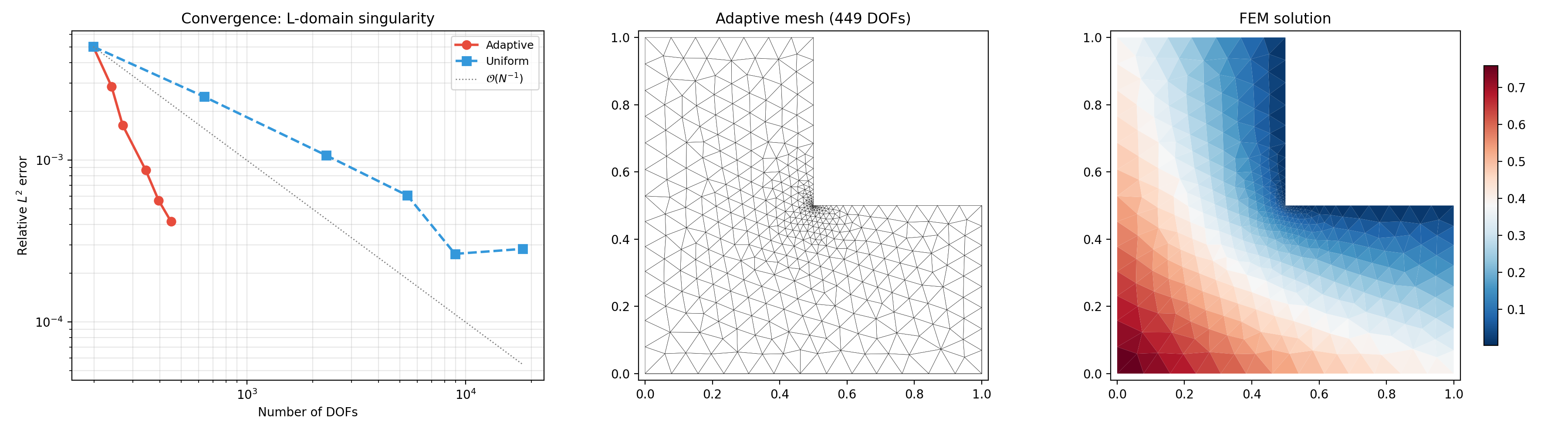
Fig. 40 Output of poisson_h_adaptivity.py regenerated with the normal-gradient-jump estimator. Left: relative \(L^2\) error vs DOF count. Middle: the final adaptive mesh with elements clustered at the re-entrant corner. Right: the FEM solution itself.

Running the examples

cd examples/poisson
python poisson.py                          # 2D, writes poisson.png
python poisson_3d.py                       # 3D, writes poisson_3d.vtu
python poisson_h_adaptivity.py             # writes poisson_h_adaptivity.png

What’s next

• Forms — the assembler base classes and the forward argument-dispatch contract used in every script above.

• Boundary Conditions — non-homogeneous Dirichlet via dirichlet_value (used in the L-shape adaptive example).

• ML Datasets — batched right-hand sides over many source terms, the natural ML data-generation extension of the basic 2D solve.

• Diffusion — same machinery, plus time stepping.