Inverse Design & Identification

TensorMesh is differentiable end to end: every step of Mesh → Assembler → SparseMatrix → Condenser → Solve is an nn.Module or a custom autograd.Function, and the linear solve carries an analytic adjoint backward (inherited from torch-sla). A loss computed on the FEM solution can therefore be back-propagated to anything upstream — a coefficient at every node, a per-element design density, a source term — without writing a single sensitivity equation by hand. The Differentiability chapter covers the mechanics; this gallery turns it into three runnable scripts in examples/inverse_design/.

They span the two flavours of “gradient through the PDE”:

• Identification — recover an unknown field from observations (coefficient_identification.py).

• Design — choose a field that optimises an objective under constraints (thermal_topology.py and compliance_topology.py).

Note

All three obtain their gradients purely from autograd. None of them implements an adjoint by hand — that is the whole point. The classical SIMP sensitivity \(\partial C/\partial \rho_e = -p\,\rho_e^{p-1}(E_{\max}-E_{\min})\, \mathbf{u}_e^{T}\mathbf{K}_0^e\mathbf{u}_e\) falls out of compliance.backward() automatically.

Coefficient-field identification — coefficient_identification.py

Recover an unknown, spatially varying diffusion coefficient \(\kappa(x)\) in

\[-\nabla\!\cdot\!\big(\kappa(x)\,\nabla u\big) = f \quad\text{in }(0,1)^2, \qquad u = 0 \text{ on }\partial\Omega,\]

from a single observed solution \(u_{\rm obs}\). The forward map is “FEM-solve given \(\kappa\)”; the loss is the L² distance to the observation; Adam descends it. We parametrise \(\kappa = 1 + \tanh\theta\) so \(\kappa\in(0,2)\) stays strictly positive (the matrix is SPD every iteration) with \(\theta\) unconstrained.

class WeightedLaplace(ElementAssembler):
    def forward(self, gradu, gradv, kappa):
        return kappa * (gradu @ gradv)

def fem_solve(kappa):
    K = WeightedLaplace.from_mesh(mesh)(point_data={"kappa": kappa}).double()
    b = Source.from_mesh(mesh)(point_data={"f": f_vals}).double()
    K_, b_ = cond(K, b)
    return cond.recover(K_.solve(b_))

theta = torch.zeros(mesh.n_points, requires_grad=True)   # kappa = 1 + tanh(theta)
optim = torch.optim.Adam([theta], lr=3e-2)
for step in range(5000):
    optim.zero_grad()
    u    = fem_solve(1.0 + torch.tanh(theta))
    loss = ((u - u_obs) ** 2).sum()
    loss.backward()                 # adjoint solve gives dLoss/dtheta
    optim.step()

Over 5000 steps the data loss falls by more than seven orders of magnitude and the recovered field matches the four-lobe ground truth almost everywhere:

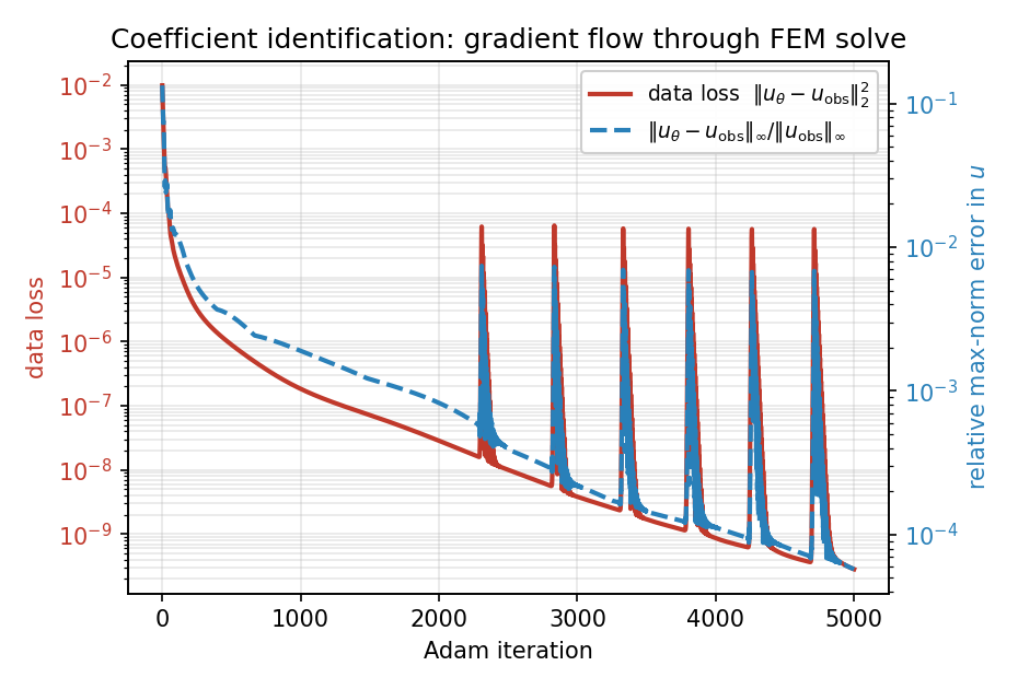
Fig. 51 Optimisation history: the data loss \(\|u_\theta - u_{\rm obs}\|_2^2\) drops to \(\sim 3\times10^{-10}\) (the periodic spikes are Adam overshooting in the ill-conditioned valley, recovered within a few steps); the relative max-norm error in \(u\) reaches \(\sim 6\times10^{-5}\).

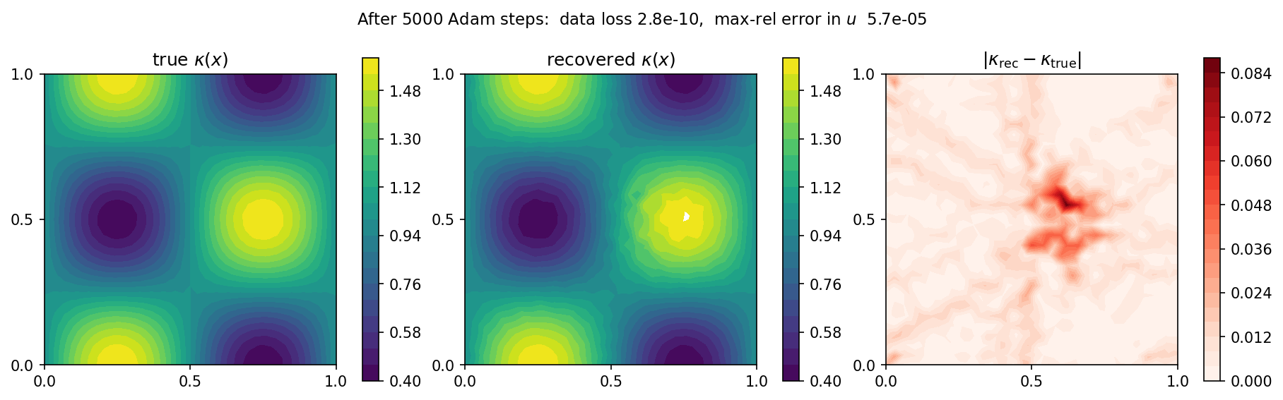
Fig. 52 True (left), recovered (middle), and absolute-error (right) coefficient fields. The only visible residual is a faint blob at the centre, where the constant source makes \(\nabla u\) vanish: with no flux there the data barely constrains \(\kappa\), so that region is recovered slowest. A smoothness penalty on \(\theta\) removes it.

Thermal-compliance topology optimization — thermal_topology.py

Distribute a fixed amount of conductive material on the unit square so as to drain heat from a central source to the cold boundary as efficiently as possible — minimise the thermal compliance \(J = \mathbf{b}^{T}\mathbf{u}\) under a hard volume cap:

\[\min_{\rho}\;\; \mathbf{b}^{T}\mathbf{u} \quad\text{s.t.}\quad \mathbf{K}(\rho)\,\mathbf{u} = \mathbf{b},\;\; \tfrac{1}{|\Omega|}\!\int_\Omega \rho \le V,\;\; \rho_{\min}\le\rho\le 1,\]

with a SIMP conductivity law \(\kappa(\rho)=\kappa_{\min}+(1-\kappa_{\min})\,\rho^{p}\) and a per-element density \(\rho\). The compliance gradient comes from autograd; the density update is the built-in OCOptimizer (Optimality Criteria with a volume-bisection step).

from tensormesh.optimizer import OCOptimizer

rho   = torch.full((n_elem,), V, requires_grad=True)
optim = OCOptimizer(rho, vf=V, move_limit=0.15)

def fem_solve(rho):
    kappa = kmin + (1.0 - kmin) * rho ** p_simp           # SIMP, per element
    K = SIMPLaplace.from_mesh(mesh)(element_data={"kappa": kappa}).double()
    b = Source.from_mesh(mesh)(point_data={"f": f_field}).double()
    K_, b_ = cond(K, b)
    return cond.recover(K_.solve(b_)), b

for step in range(60):
    optim.zero_grad()
    u, b = fem_solve(rho)
    compliance = (b * u).sum()      # J = b^T u
    compliance.backward()           # autograd populates rho.grad
    optim.step()                    # OC update + volume bisection

The optimal layout is a “thermal cross” connecting the hot centre to the four cold mid-edges; compliance drops about \(8.6\times\) (\(5.9\times10^{-3} \to 6.9\times10^{-4}\)) while the volume fraction is held at \(0.4\) exactly:

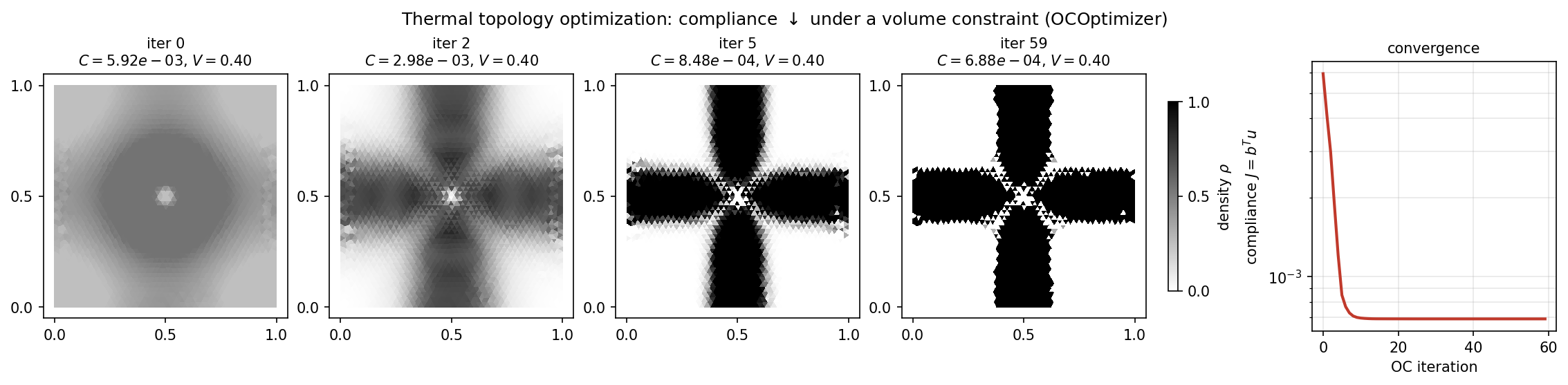
Fig. 53 Density evolution over 60 OC steps (iteration 0 is the uniform \(\rho = V\) start) and the compliance history. The cross has emerged by iteration 5 and sharpens into a near 0/1 design by the end.

This is the scalar/heat counterpart of the structural problem below: identical “autograd sensitivity + density update” pattern, different physics and a different optimiser.

Structural compliance topology optimization — compliance_topology.py

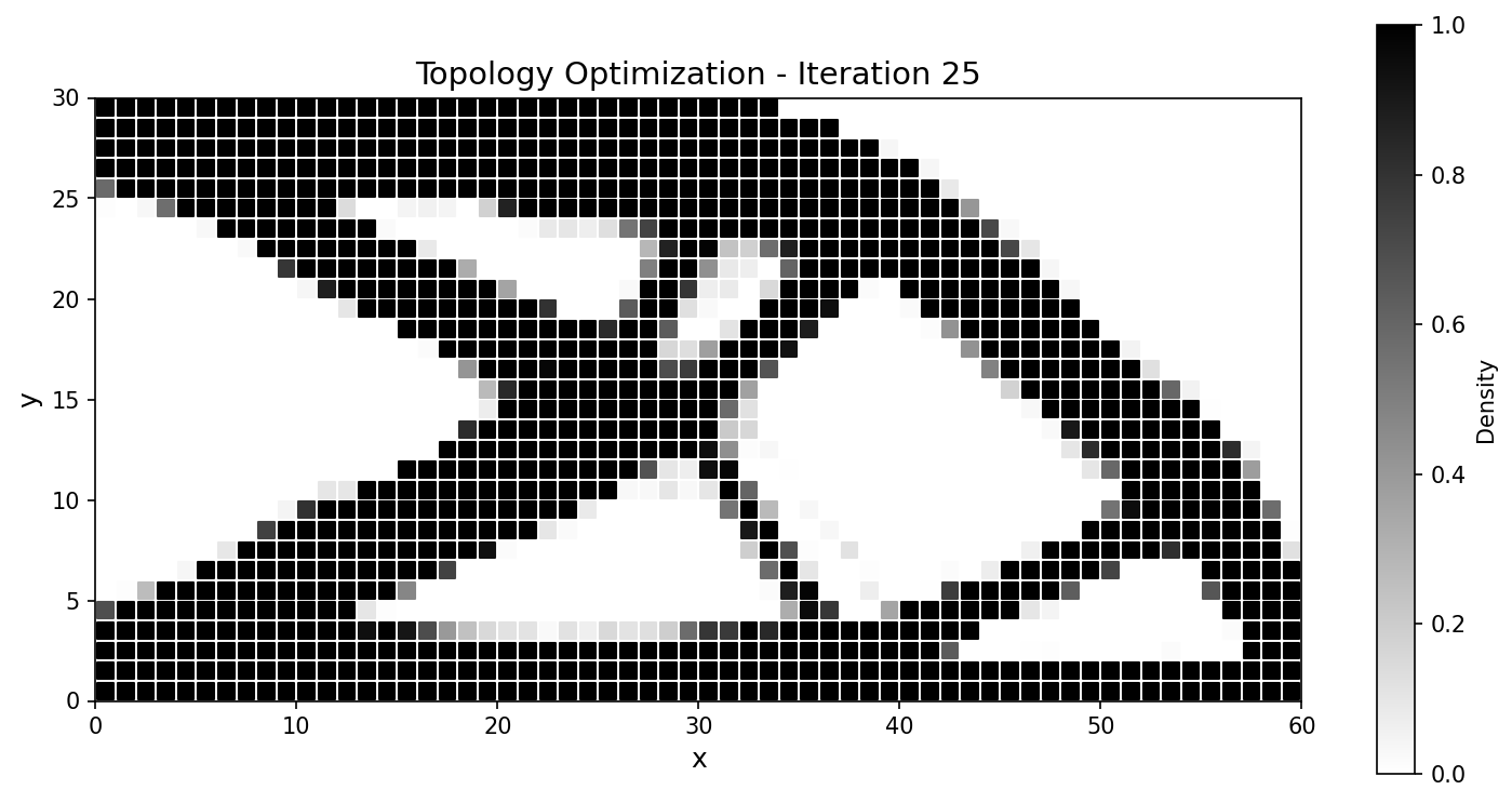
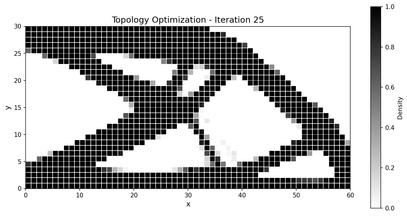
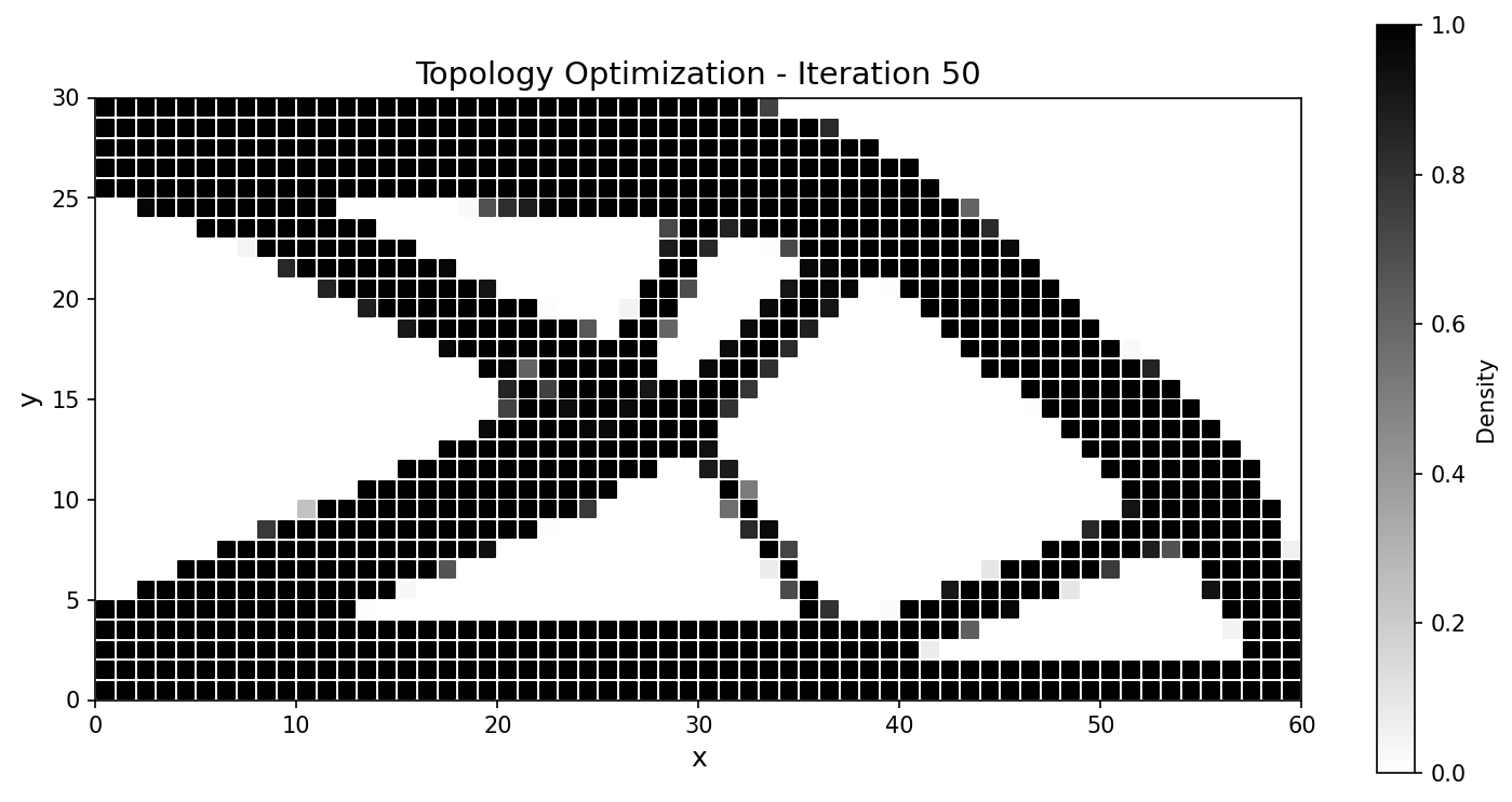
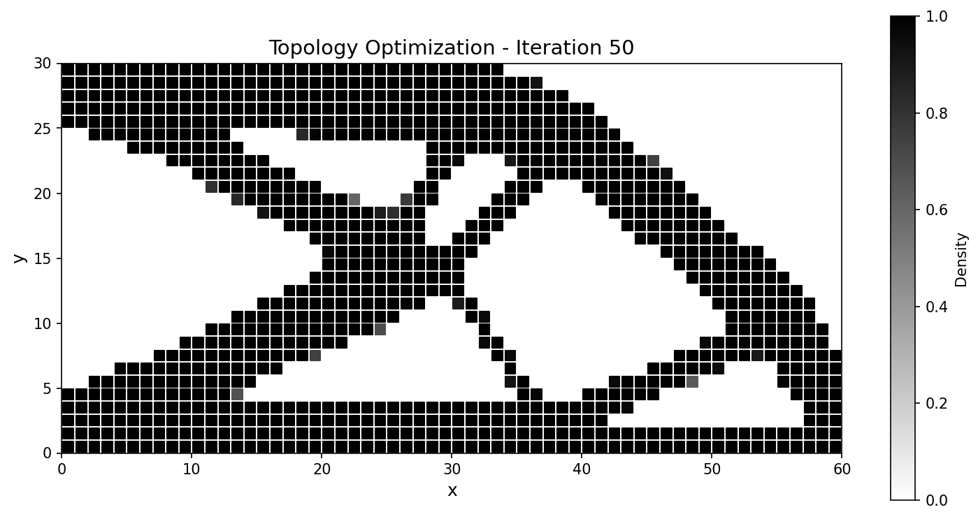
The classical 2D cantilever: minimise structural compliance under a volume constraint, SIMP density interpolation, MMA (Method of Moving Asymptotes) updates with a density filter. It is set up to match a JAX-FEM reference problem for a head-to-head comparison.

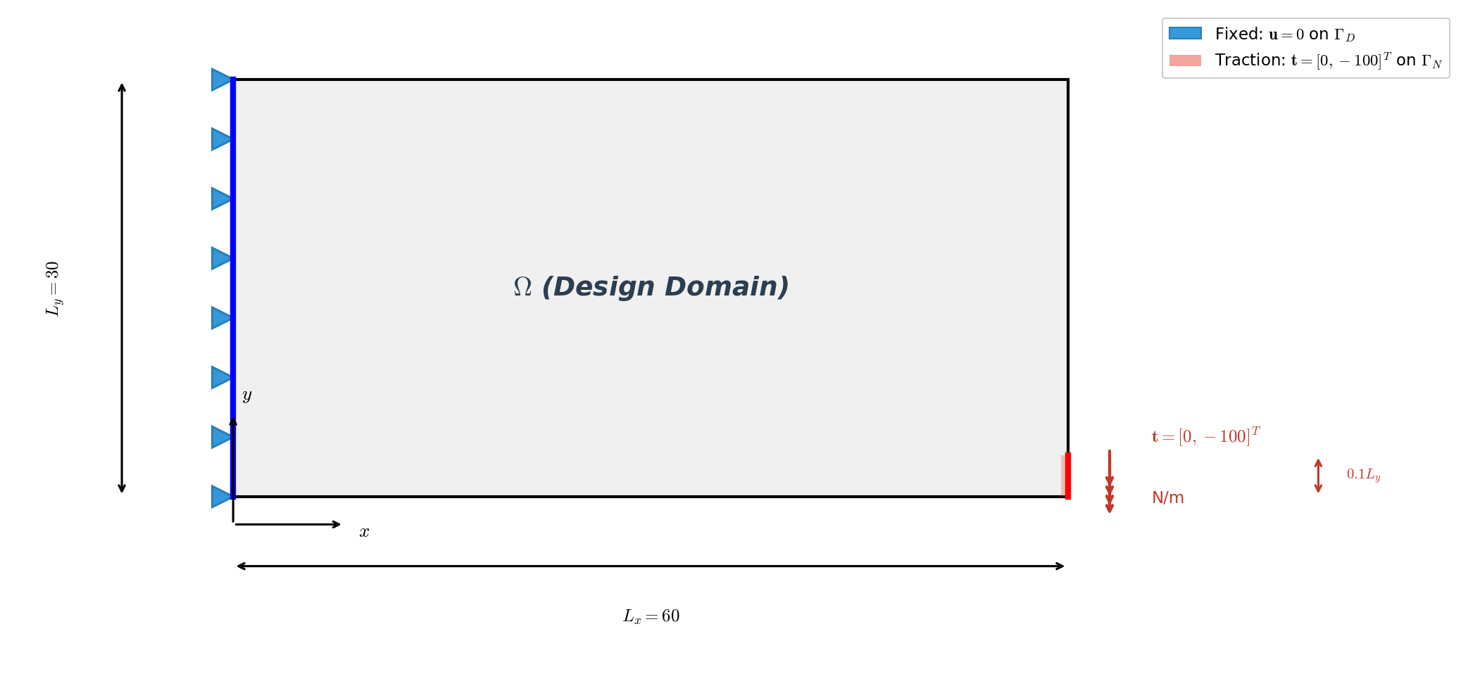
Setup. Domain \(60\times30\) with \(60\times30\) QUAD4 elements (1891 nodes, 1800 elements); left edge clamped (\(\mathbf{u}=\mathbf{0}\) at \(x=0\)); a downward traction \(\mathbf{t}=[0,-100]^{T}\) on the bottom-right corner; plane-stress material with \(E_{\max}=70\,000\), \(E_{\min}=70\), \(\nu=0.3\), SIMP penalty \(p=3\), target volume fraction \(\bar v = 0.5\).

\[\min_{\rho}\; C(\rho) = \mathbf{u}^{T}\mathbf{K}(\rho)\,\mathbf{u} \quad\text{s.t.}\quad \mathbf{K}(\rho)\mathbf{u} = \mathbf{F},\;\; \tfrac{1}{|\Omega|}\!\int_\Omega\rho \le \bar v,\;\; 0 < \rho_{\min}\le\rho\le 1, \qquad E(\rho) = E_{\min} + \rho^{p}\,(E_{\max}-E_{\min}).\]

The plane-stress stiffness integrand is written directly in the assembler’s forward; rho enters per element via element_data, and the compliance gradient is again just compliance.backward():

class SIMPStiffnessAssembler(ElementAssembler):
    def __post_init__(self, E_max=70e3, E_min=70.0, nu=0.3, penal=3.0):
        self.E_max, self.E_min, self.nu, self.penal = E_max, E_min, nu, penal

    def forward(self, gradu, gradv, rho):
        E = self.E_min + rho ** self.penal * (self.E_max - self.E_min)
        D11, D12 = E / (1 - self.nu**2), self.nu * E / (1 - self.nu**2)
        D33 = E / (2 * (1 + self.nu))
        gux, guy = gradu[0], gradu[1]
        gvx, gvy = gradv[0], gradv[1]
        K00 = D11 * gux * gvx + D33 * guy * gvy
        K01 = D12 * gux * gvy + D33 * guy * gvx
        K10 = D12 * guy * gvx + D33 * gux * gvy
        K11 = D11 * guy * gvy + D33 * gux * gvx
        return torch.stack([torch.stack([K00, K01]), torch.stack([K10, K11])])

for epoch in range(max_iters):
    rho_var = rho.clone().requires_grad_(True)
    K = K_asm(mesh.points, element_data={"rho": rho_var})
    K_, F_ = condenser(K, F)
    u = condenser.recover(K_.solve(F_, backend="scipy"))
    compliance = u @ F
    compliance.backward()                 # dC/drho via autograd
    optimizer.step(dc=rho_var.grad, dv=torch.ones_like(rho) / n_elem)

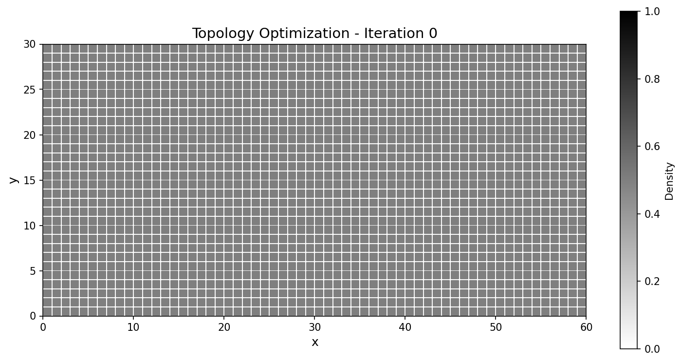
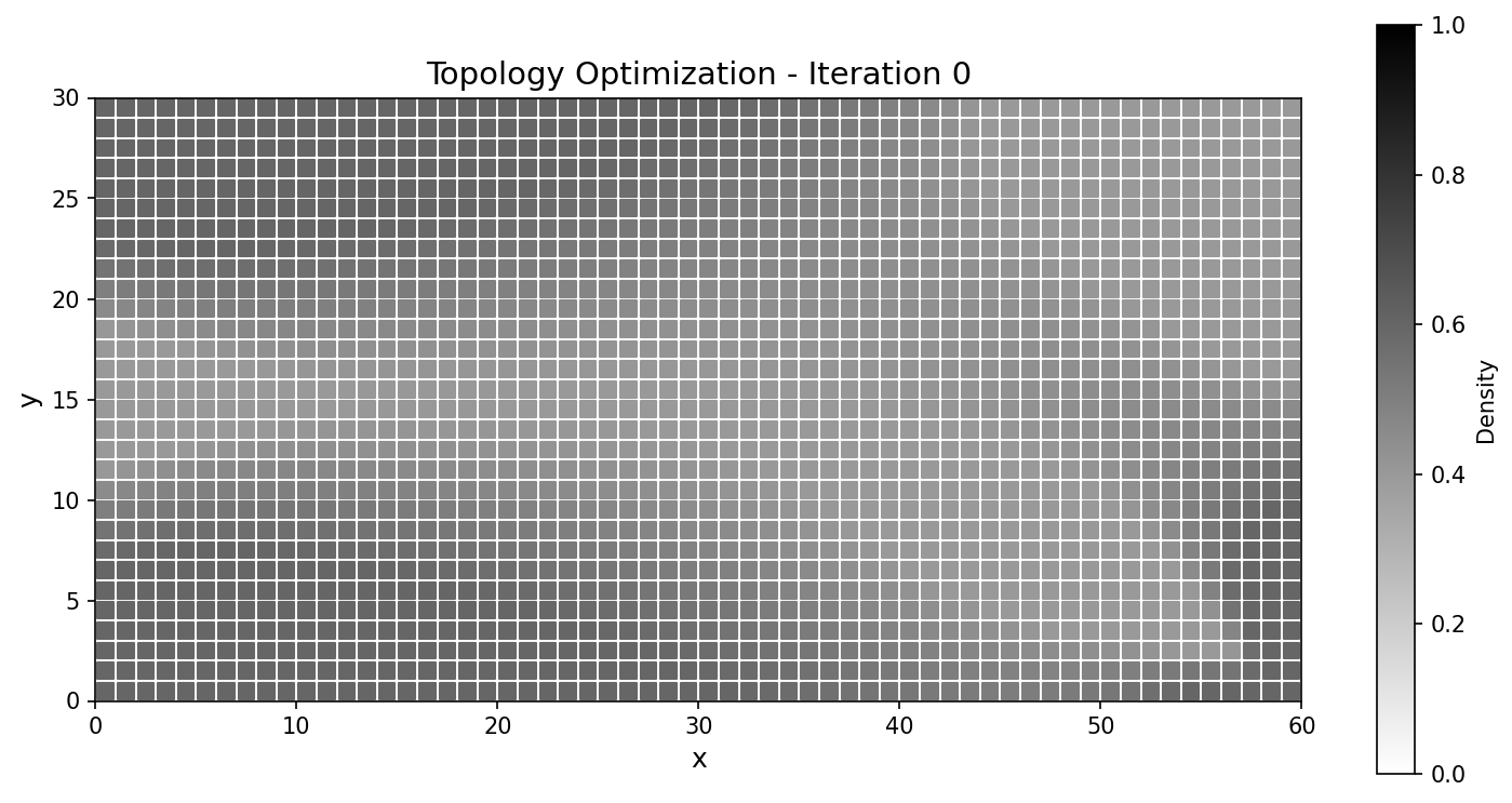
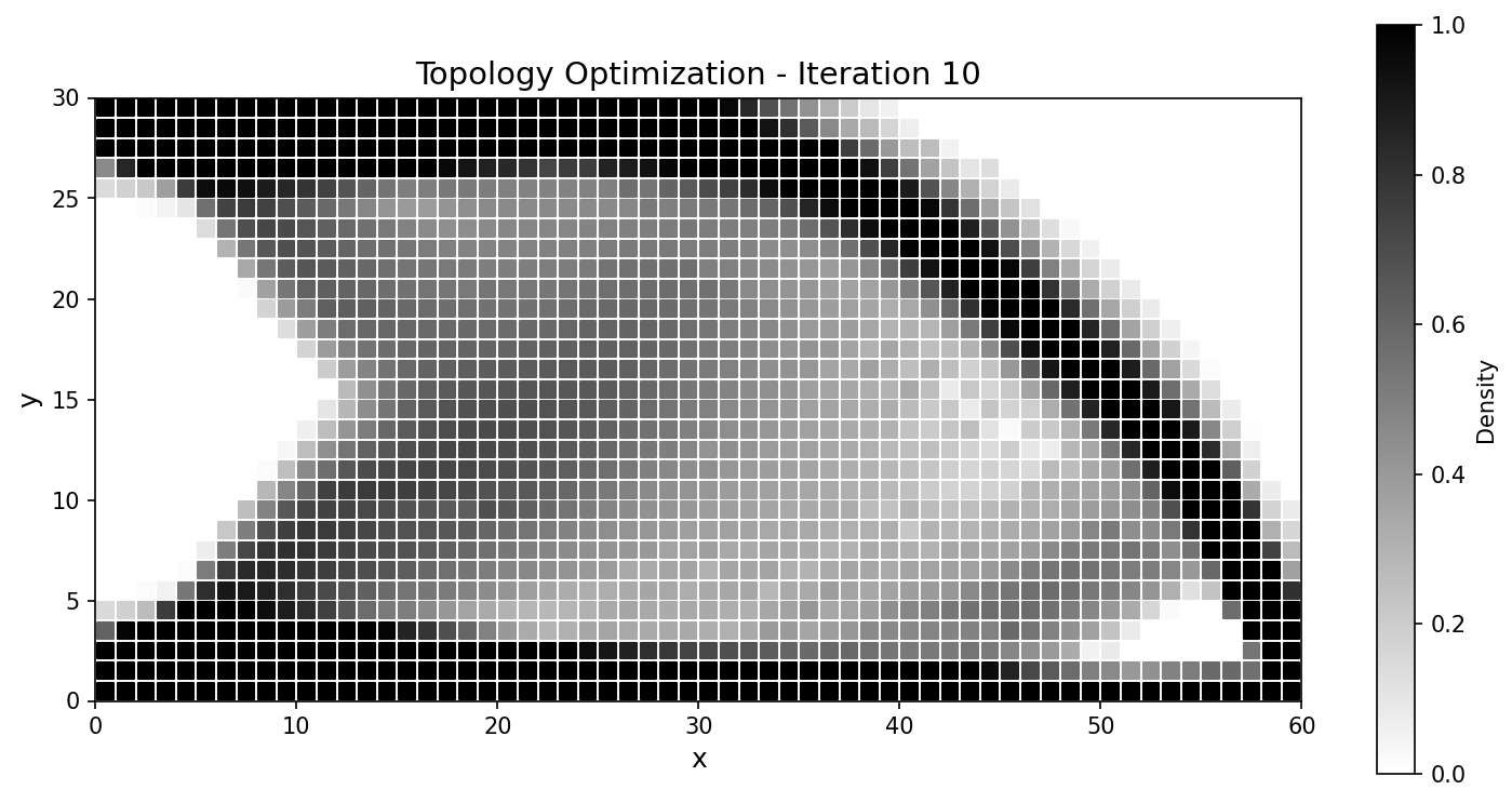
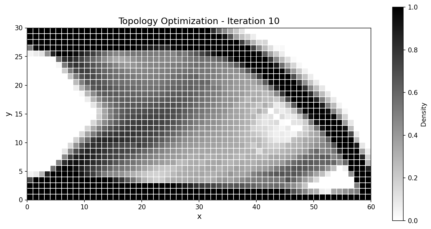
The optimizer converges to the canonical cantilever truss, tracking the JAX-FEM reference closely:

Iter	JAX-FEM	TensorMesh
0
10
25
50

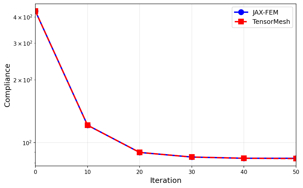
Fig. 54 Compliance histories agree across the run; the final designs match to a fraction of a percent.

Table 1 Accuracy and timing (51 iterations) vs. the JAX-FEM reference

Metric	JAX-FEM	TensorMesh	Note
Final compliance	84.03	83.75	0.33 % difference
Volume fraction	0.500	0.500	matched
Total time	31.13 s	8.35 s	3.7× faster

Note

This example depends on the local mma_optimizer.py (a small MMA implementation) and on meshio / tqdm for VTK export and the progress bar. The lighter thermal_topology.py above uses the built-in OCOptimizer and has no extra dependencies.

Running the examples

cd examples/inverse_design

python coefficient_identification.py    # ~1 min CPU -> coefficient_id_*.png
python thermal_topology.py              # a few seconds -> thermal_topology.png
python compliance_topology.py           # cantilever; writes output/

Each accepts --device cuda and a few problem-size flags (--n-iter, --chara-length, --vf); pass -h for the list.

What’s next

• Differentiability — the adjoint backward, the full cost/correctness story, and how to wire a neural network into any of these loops.

• Sparse Solvers — the autograd-aware SparseMatrix.solve and nonlinear_solve behind every solve here.

• ML Datasets — batched forward solves for ML training data, the other side of differentiable FEM.