Elements and Quadrature
Every entry in cells is keyed by an element
type string — "triangle", "hexahedron27", "wedge", and so
on — that maps to one of the seven reference shapes in
tensormesh.element. The element classes carry the basis-function
definitions and quadrature rules that the assembler uses internally;
you rarely call them directly, but understanding what they expose makes
the rest of the pipeline (assembly, IO, higher-order solves) less
mysterious.
This page is laid out in two parts. First, the catalog of supported
types and the high-level rule for going from order=1 to higher-order
solves. Second, a guided tour through the reference → physical
pipeline that turns a static reference-element definition into the
per-element shape values, gradients, and integration weights an
assembler actually consumes.
Supported element types
TensorMesh ships seven reference shapes covering 1D, 2D, and 3D, with linear and higher-order variants for each:
Class |
Dim |
Linear type string |
Higher-order type strings |
|---|---|---|---|
1D |
|
|
|
2D |
|
|
|
2D |
|
|
|
3D |
|
|
|
3D |
|
|
|
|
3D |
|
|
3D |
|
|
The mapping between strings and dimensions / orders is exposed as two plain dicts:
from tensormesh import element_type2order, element_type2dimension
element_type2order["triangle6"]      # 2
element_type2dimension["hexahedron"] # 3
A reverse map element_type2element returns the class:
from tensormesh.element import element_type2element
element_type2element("hexahedron27")  # tensormesh.Hexahedron
Type-string naming follows meshio: the lowercase shape (triangle)
plus the basis-node count for higher-order variants (triangle6,
hexahedron27). Note one inconsistency carried over from meshio —
the 3D triangular prism is the class Prism but
the string "wedge".
Higher-order elements
Pass order=2 (or 3, …) to a built-in mesh generator:
from tensormesh import Mesh

tri  = Mesh.gen_rectangle(chara_length=0.1, order=1)  # "triangle"
tri6 = Mesh.gen_rectangle(chara_length=0.1, order=2)  # "triangle6"
hex27 = Mesh.gen_cube(chara_length=0.2, order=2)      # "hexahedron27"
The element type string in mesh.cells updates accordingly, and
every assembler downstream picks up the higher-order basis without
any further configuration.
The pipeline: from reference shape to physical integration
Conceptually the element layer answers one question: given a weak form to integrate over a mesh, where are the quadrature points, what are the shape-function values and gradients there, and what is the integration weight? It does this by composing seven static reference-element definitions with the physical-space connectivity of your mesh. The overall flow is:
Element subclass (Triangle / Hexahedron / ...) — static topology
        │
        ▼
get_basis(order)          : Lagrange nodes on the reference element   [N_b, D]
get_polynomial(order)     : polynomial space (P_k or Q_k or ...)
        │
        ▼   (Vandermonde inversion, done once and cached)
get_basis_fns(order)      : hat functions  φ_b(ξ)                     [N_b]
get_basis_grad_fns        : reference-space gradients ∂φ/∂ξ
        │
        ▼
get_quadrature(order)     : reference-element Gauss points + weights
        │
        ▼   (compose the two layers above)
eval_shape_val            : φ_b(ξ_q)                                   [N_q, N_b]
                             ↑ mesh-independent, shared across cells

eval_cell_jacobian        : J(ξ_q; e)                                  [N_e, N_q, D, D]
eval_shape_grad           : ∇_x φ_b(ξ_q; e)                            [N_e, N_q, N_b, D]
                             ↑ first place the physical coordinates enter

        │
        ▼
Transformation(points, elements, type)
    ├ shape_val      = φ        at Gauss points (reference, cached buffer)
    ├ shape_grad     = ∇_x φ    at Gauss points (physical)
    ├ jacobian       = J
    ├ JxW            = |det J| · w           ← volume-integral measure
    ├ facet_*        : same quantities but on each facet
    └ nanson_scale / FxW                     ← surface-integral measure
The rest of this section walks through every box and shows what the
returned tensors actually look like. All examples use
Triangle because it is the cheapest to print, but
the structure is identical for the other six shapes.
Step 0 — Reference-element topology
Each subclass carries a handful of class-level torch.Tensor /
tuple attributes that pin down the reference geometry. Nothing
here depends on order — these are just the corners of the
reference shape and how they connect:
from tensormesh import Triangle

Triangle.points                                  # vertex coordinates
# tensor([[0., 0.],
#         [1., 0.],
#         [0., 1.]])
Triangle.edge                                    # vertex-pair connectivity
# tensor([[1, 2],
#         [0, 2],
#         [0, 1]])
Triangle.face                                    # tuple of vertex tuples
# ((0, 1, 2),)
Triangle.dim, Triangle.n_vertex, Triangle.n_edge
# (2, 3, 3)
Two derived attributes worth knowing about:
is_mix_facet is True for
Prism and Pyramid (whose
facets come in two shapes), and otherwise False;
get_facet_type() returns the facet element
class (Line for a triangle, Triangle for a tetrahedron, the
tuple (Triangle, Quadrilateral) for a prism).
Step 1 — Lagrange nodes (get_basis)
get_basis() picks where the interpolation
nodes sit on the reference element for a given polynomial order. The
convention is vertex nodes first, then edge nodes, then face/interior
nodes — see Gmsh / VTK ↔ TensorMesh node ordering for the visual companion
across all seven shapes.
Triangle.get_basis(order=1)
# tensor([[0., 0.],    # vertex nodes
#         [1., 0.],
#         [0., 1.]])
Triangle.get_basis(order=2)
# tensor([[0.0, 0.0],  # vertex nodes (3)
#         [1.0, 0.0],
#         [0.0, 1.0],
#         [0.5, 0.5],  # edge midpoints (3)
#         [0.0, 0.5],
#         [0.5, 0.0]])
The output shape is [N_b, D] with \(N_b = (p+1)(p+2)/2\) for
simplex shapes and \((p+1)^d\) for tensor-product shapes (quad /
hex). Every other step in the pipeline indexes into this layout, so it
is the single source of truth for “what does basis function b mean?”
Step 2 — Polynomial space (get_polynomial)
get_polynomial() returns the polynomial space
the shape functions live in, as a
Polynomial. The space depends on the
shape: simplex elements use the full \(P_k\) (terms with total
degree \(\le k\)); tensor-product elements use \(Q_k\) (each
coordinate exponent \(\le k\)); the prism uses its own ad-hoc space.
The pyramid skips this step: no polynomial space is conforming on it, so
tensormesh.Pyramid.get_basis_fns() builds a rational basis
directly (PyramidBasisFns).
Triangle.get_polynomial(order=1)
# 1 + x + y                       (P_1 in 2D, 3 terms)
Triangle.get_polynomial(order=2)
# 1 + x + y + x^2 + xy + y^2      (P_2 in 2D, 6 terms)
You usually never call this directly — get_basis_fns() invokes
it for you. The hook is meant to be overridden by people adding a new
element type, so that the base class can synthesise the Lagrange basis
on top of a custom polynomial space.
Step 3 — Hat functions (get_basis_fns, get_basis_grad_fns)
get_basis_fns() combines the previous two —
Lagrange nodes plus polynomial space — into the basis function set.
Internally TensorMesh evaluates the polynomial-space terms at the
basis nodes, inverts the resulting Vandermonde matrix, and pushes the
coefficients into a Polynomials (batched
polynomial) object. The output satisfies the Lagrange property
\(\phi_b(\boldsymbol{\xi}_{b'}) = \delta_{bb'}\).
fns = Triangle.get_basis_fns(order=1)
print(fns)
# [1 -x -y,
#  x,
#  y]
fns.shape, fns.n_vars, fns.n_terms
# ((3,), 2, 3)

# Reference-space gradient ∂φ_b / ∂ξ_i  — already symbolic.
grad_fns = Triangle.get_basis_grad_fns(order=1)
print(grad_fns)
# [[-1, 1, 0],     # ∂/∂x
#  [-1, 0, 1]]     # ∂/∂y
grad_fns.shape
# (2, 3)             # [dim, n_basis]
The result of get_basis_fns() is mesh-independent — every
element in the mesh, regardless of physical shape, uses the same
\(\phi_b(\boldsymbol{\xi})\). This is the entire point of the
reference-element trick.
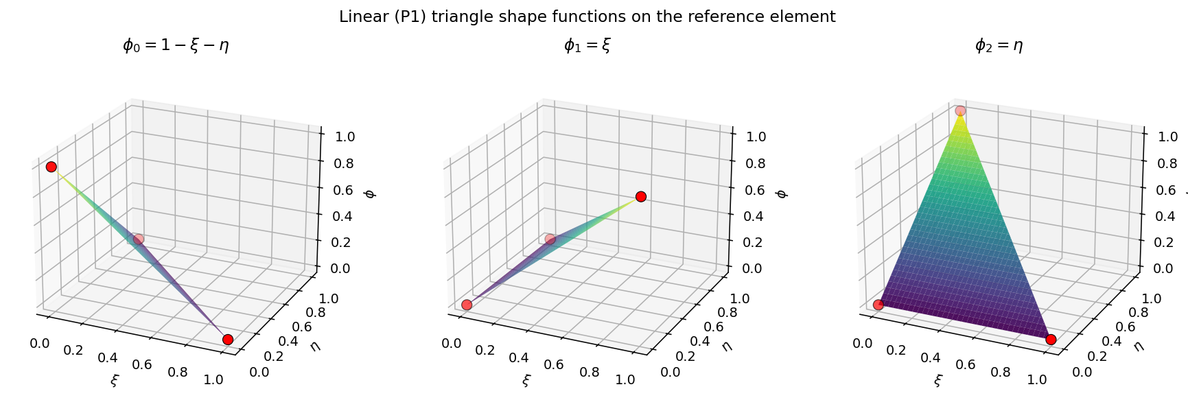
Fig. 6 The three P1 shape functions on the reference triangle. Each \(\phi_b\) equals 1 at vertex b (red marker) and decays linearly to 0 at the other two vertices.
For higher-order surface plots on every supported shape, see
Basics & Visualization (section “Shape functions”). Internally
the example_gallery scripts call exactly the
get_basis_fns() you just saw — there is no
separate plotting code path.
Step 4 — Reference quadrature (get_quadrature)
get_quadrature() returns a Gauss-type rule on
the reference element — weights of shape [N_q] and points of shape
[N_q, D]. The order argument is the quadrature order, not the
basis order; pick it large enough to integrate your weak form exactly.
As a rule of thumb, quadrature_order = 2 * basis_order is enough
for most bilinear forms on Laplace-type problems.
w, q = Triangle.get_quadrature(order=2)
w     # tensor([0.1667, 0.1667, 0.1667])     (sum = 1/2 = |reference triangle|)
q     # tensor([[0.1667, 0.1667],
      #         [0.6667, 0.1667],
      #         [0.1667, 0.6667]])
Triangle, quad, hex, tet, pyramid, prism each pick a different rule
family; see tensormesh/element/quadrature.py for the tables.
Step 5 — Reference shape values (eval_shape_val)
eval_shape_val() composes Step 3 (basis
functions) with Step 4 (quadrature points): the resulting matrix has
entry \([q, b] = \phi_b(\boldsymbol{\xi}_q)\). This is still
purely reference-element data — no mesh has been touched.
phi = Triangle.eval_shape_val(quadrature_order=2, order=1)
phi.shape
# torch.Size([3, 3])   # [N_q=3, N_b=3]
phi
# tensor([[0.6667, 0.1667, 0.1667],   # rows sum to 1 (partition of unity)
#         [0.1667, 0.6667, 0.1667],
#         [0.1667, 0.1667, 0.6667]])
Every element of every mesh, no matter its physical shape, reuses this single \([N_q, N_b]\) matrix. This is the source of the FEM speed-up over collocation methods — you build it once and broadcast it across all elements during assembly.
Step 6 — Cell Jacobian and physical gradients
Now the mesh enters. For each element \(e\), the isoparametric map
sends the reference element \(\hat K\) to the physical element \(K^e\), where \(\mathbf{x}^e_b\) are the physical coordinates of element e’s basis nodes. Its Jacobian \(\mathbf{J}^e_q = \partial \mathbf{x}^e / \partial \boldsymbol{\xi}\), evaluated at quadrature point \(q\), is
eval_cell_jacobian() computes exactly this
sum across the whole mesh:
import torch
from tensormesh import Triangle

# Three different physical triangles sharing the same reference shape.
coords = torch.tensor([
    [[0., 0.], [1., 0.], [0., 1.]],   # canonical
    [[0., 0.], [2., 0.], [0., 1.]],   # stretched in x by 2
    [[0., 0.], [1., 0.], [1., 2.]],   # sheared
])
_, q = Triangle.get_quadrature(order=2)

J = Triangle.eval_cell_jacobian(q, coords, basis_order=1)
J.shape                              # torch.Size([3, 3, 2, 2])  [N_e, N_q, D, D]
J[0, 0]; J[1, 0]; J[2, 0]
# element 0: identity                element 1: diag(2, 1)     element 2: [[1,0],[1,2]]
Physical-space gradients of the shape functions are then obtained by
the chain rule \(\nabla_{\!x}\phi_b = \mathbf{J}^{-T}\nabla_{\!\xi}\phi_b\),
which eval_shape_grad() packages together
with the Jacobian it had to compute anyway:
grad, J = Triangle.eval_shape_grad(coords, basis_order=1)
grad.shape                           # [N_e, N_q, N_b, D]

grad[0, 0]                           # canonical triangle
# tensor([[-1., -1.],                # ∇φ_0
#         [ 1.,  0.],                # ∇φ_1
#         [ 0.,  1.]])               # ∇φ_2

grad[1, 0]                           # stretched triangle: x-derivative halved
# tensor([[-0.5000, -1.0000],
#         [ 0.5000,  0.0000],
#         [ 0.0000,  1.0000]])
This is the first place in the pipeline where the physical
coordinates element_coords enter. Everything before this point
(get_basis, get_basis_fns, eval_shape_val) was pure
reference-element data; everything after it depends on the mesh
geometry.
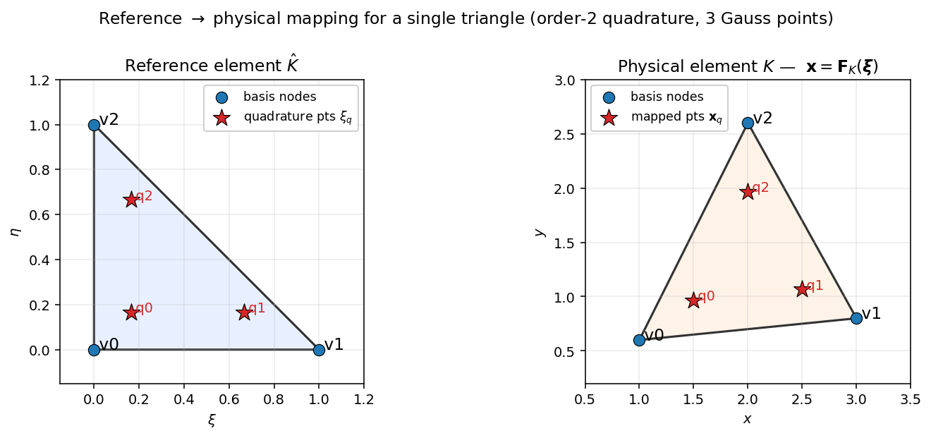
Fig. 7 Step 6 visualised on a single triangle. Left: reference element \(\hat K\) with its three order-2 Gauss points. Right: a stretched, translated physical triangle \(K\). The Gauss points are mapped through the isoparametric map \(\mathbf{F}_K\); values \(\phi_b(\boldsymbol{\xi}_q)\) reused unchanged from Step 5 are now tied to the physical points \(\mathbf{x}_q\) for integration. The Jacobian \(\mathbf{J}\) of this map drives both the gradient transform and the \(\lvert\det\mathbf{J}\rvert\) volume factor in the next step.
Step 7 — Transformation: the cached package
In practice you never call eval_* directly. Instead you instantiate
a Transformation, which lazily wires together
every step of the pipeline and caches the results as
torch.nn.Module buffers (so .to(device) / .double() /
.cuda() Just Work).
import tensormesh as tm

mesh = tm.Mesh.gen_rectangle(chara_length=0.4)         # 26 triangles, 20 nodes
t = tm.Transformation(
    mesh.points,
    mesh.cells["triangle"],
    element_type="triangle",
    quadrature_order=2,
)

t.shape_val.shape                            # [N_q, N_b]            = [3, 3]
t.shape_grad.shape                           # [N_e, N_q, N_b, D]    = [26, 3, 3, 2]
t.jacobian.shape                             # [N_e, N_q, D, D]      = [26, 3, 2, 2]
t.JxW.shape                                  # [N_e, N_q]            = [26, 3]

# Integral of 1 over the unit square — should equal 1.
t.JxW.sum().item()
# 1.0000000000000002
The named attributes correspond directly to the pipeline:
Attribute |
Math |
Shape |
|---|---|---|
\(\phi_b(\boldsymbol{\xi}_q)\) |
|
|
\(\nabla_{\!x}\phi_b(\mathbf{x}^e_q)\) |
|
|
\(\mathbf{J}^e_q\) |
|
|
\(\lvert\det\mathbf{J}^e_q\rvert\, w_q\) |
|
The reason the pipeline matters even when you only use
Transformation is that each attribute has a
fixed cost and a fixed memory footprint, both controlled by exactly
two knobs: the element type (sets \(N_b\)) and the quadrature
order (sets \(N_q\)). When you write a custom assembler and reach
for t.shape_grad, you now know that what you are holding is a
\([N_e, N_q, N_b, D]\) tensor built by composing
get_basis_grad_fns (Step 3) with get_quadrature (Step 4) and
the per-element inverse Jacobian (Step 6).
For shorthand TensorMesh aliases phi := shape_val, gradphi :=
shape_grad, J := jacobian, G := jacobian, GxW := JxW —
useful when transcribing weak forms directly from the math.
Facet quantities
Surface integrals follow the same pipeline but the reference element
becomes the facet (an edge in 2D, a face in 3D), and the volume
measure \(\lvert\det\mathbf{J}\rvert w\) becomes the Nanson area
scale \(\lvert\det\mathbf{J}_K\rvert \lVert\mathbf{J}_K^{-T}
\mathbf{n}\rVert w\). Transformation exposes the
facet analogues with the same naming pattern:
Attribute |
Math |
Notes |
|---|---|---|
\((w^f_q, \boldsymbol{\xi}^f_q)\) |
Facet-local Gauss rule |
|
\(\phi_b(\boldsymbol{\xi}^f_q)\) |
Cell shape fns evaluated on each facet |
|
\(\nabla_{\!x}\phi_b(\mathbf{x}^f_q)\) |
Chain-ruled through the cell Jacobian |
|
|
facet-tangent Jacobian \(\mathbf{J}_f\) |
Maps facet-local to physical coords |
|
\(\lvert\det\mathbf{J}\rvert\,\lVert\mathbf{J}^{-T}\mathbf{n}\rVert\, w\) |
Outward-facing surface measure |
\(\lvert\mathbf{J}_f\rvert\, w\) |
Surface-integration shortcut |
For elements with mixed facet types (Prism,
Pyramid) every one of these attributes returns a
tuple — triangular-facet quantities first, quadrilateral-facet
quantities second. The high-level FacetAssembler in
tensormesh.assemble handles the case-split for you.
The ordering convention
TensorMesh stores connectivity for tensor-product shapes
(Quadrilateral, Hexahedron)
in lexicographic order — the order that matches the underlying
tensor-product polynomial layout. Gmsh and VTK use a different
convention. The two are not interchangeable for higher-order or
tensor-product elements: feeding Gmsh-ordered hex27 connectivity
straight into the assembler produces silently-broken basis
evaluations.
The single conversion point is reorder():
Element.reorder(elements, to_gmsh=False)— Gmsh/VTK → TensorMesh (used when reading external meshes).Element.reorder(elements, to_gmsh=True)— TensorMesh → Gmsh/VTK (used when writing.vtk/.vtufiles).
You almost never call reorder() directly. The
high-level paths do it for you:
The built-in mesh generators emit TensorMesh ordering already.
read()andfrom_meshio()acceptreorder=Trueto convert on ingest.save()auto-detects.vtk/.vtuoutputs and reorders for you.
If you build a mesh from raw arrays
(Mesh(meshio_obj, reorder=True)) the same flag controls the
behavior — pass reorder=True when the source uses Gmsh/VTK
convention. The example gallery has a side-by-side comparison for
every element type at orders 2–4: see Gmsh / VTK ↔ TensorMesh node ordering.
Adding a new element type
Subclassing Element is the supported extension
path, and the pipeline above also tells you which hooks you need to
override:
get_polynomial()— Step 2, the polynomial space your new element lives in.get_basis()— Step 1, the interpolation-node coordinates.get_quadrature()/get_facet_quadrature()— Step 4 and its facet variant.get_facet_type(),get_facet()— facet topology and basis-index mapping.get_gmsh_permutation()— only if you want the element to round-trip through Gmsh / VTK files.
The base class derives Steps 3, 5, 6, and 7 from those overrides
automatically. The existing seven shapes in
tensormesh/element/element.py are short, self-contained templates;
the low-level helpers used inside those overrides
(Polynomial, basis-node generators,
quadrature factories) live under Extension internals.
What’s next
Forms — write a weak form against the basis tensors that these elements supply.
Meshes — generators, I/O, and the
reorder=Truecalling pattern in context.Example Gallery — working examples on triangular, quad, tet, and hex meshes (including high-order).