Batched Workflows¶

“Batched” means three different things in TensorMesh, and they operate at different layers of the pipeline. Picking the right one for your problem matters more than turning every knob at once. This chapter walks through the three axes, then gives the canonical “same mesh, many sources” recipe with end-to-end numbers measured on the development workstation.

Three axes of batching¶

Axis	Where it lives	When to reach for it
Memory chunking	`Assembler(batch_size=N)`	One assembly that doesn’t fit in GPU memory.
Batched right-hand sides	`K.solve(B)` with `B` of shape `[n_dof, n_batch]`	Many loads, one mesh, one stiffness matrix.
Multi-problem datasets	`tensormesh.dataset`	ML training data: many `(K_i, b_i)` pairs.

What is not built in: vmap-style assembly that vectorises K construction across many parameter values. If you need that, loop in Python or wrap your assembler call in torch.vmap manually – see What’s not built in below.

Axis 1 – Memory chunking with `batch_size`¶

A single ElementAssembler call holds the per-element, per-quadrature-point integrand tensor in memory. For fine meshes or high-order elements that tensor can be too large. The batch_size argument splits the quadrature dimension into chunks, accumulating the contribution one chunk at a time:

K = LaplaceElementAssembler.from_mesh(mesh)(batch_size=4)

The result is bit-identical (to machine precision) to the un-chunked call – batch_size is purely a memory knob. Default is -1 (no chunking, fastest if memory allows).

The figure below assembles the same operator on a quadratic-triangle mesh with about \(1.9\times10^{5}\) nodes on the GPU, at quadrature order 5 (\(n_q = 7\) points per element). Shrinking batch_size from the full integrand down to one quadrature point at a time drops peak memory from 810 MB to 271 MB – a 3x reduction – at essentially no extra time:

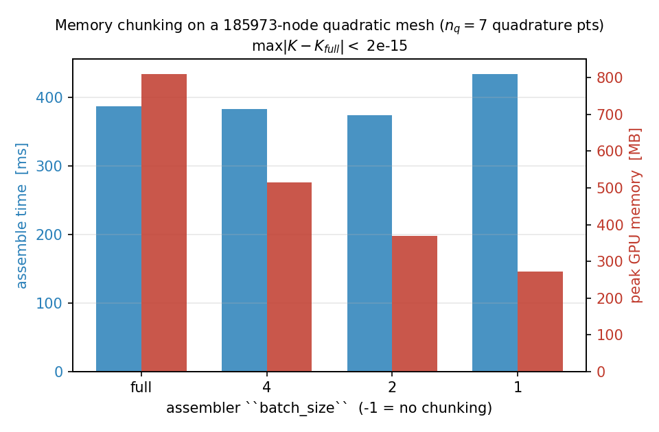
../_images/memory_chunking.png — Fig. 13 Assembly time (blue) and peak GPU memory (red) versus the `batch_size` chunk knob on a quadratic triangle mesh (185 973 nodes, \(n_q = 7\)). Peak memory falls from 810 MB (un-chunked) to 271 MB (one quadrature point per chunk); every setting produces a stiffness matrix that differs from the un-chunked reference by less than \(2 \times 10^{-15}\) in max-norm.¶

Two things temper the knob – and explain why a careless benchmark can look flat:

It only bites while batch_size \(< n_q\). Since n_batch = ceil(n_q / batch_size), any batch_size at or above the quadrature-point count collapses to a single chunk – that is, no chunking at all. At the default quadrature order an order-2 triangle has only \(n_q = 3\) points, so there is very little room to chunk; raising the quadrature order (or using high-order / vector elements) grows the transient integrand and gives the knob more to work on – which is why the figure above uses order 5.
There is a floor it cannot touch. The assembled matrix values, their int64 row/column index buffers, and the per-element accumulator [n_elem, n_basis, n_basis] are all proportional to the element count and stay resident regardless of batch_size. Chunking only pays off when the transient integrand [n_elem, n_q, n_basis, n_basis] is the dominant allocation; scaling up the mesh alone does not help, because the floor grows with it.

A typical recipe: start with the default; if you OOM, halve batch_size (down to 1) until the assembly fits.

This axis has nothing to do with batching across problems. The result is one matrix, not a batch of matrices.

Note

batch_size chunks one assembly on a single device. When the stiffness matrix is too large for one GPU even chunked, TensorMesh also has a multi-GPU distributed assembly path – currently a beta / research-grade feature; see Distributed FEM for the building blocks. A future release will align distributed assembly with the distributed linear solver in torch-sla, closing the loop on truly large-scale DOF counts end-to-end.

Axis 2 – Batched right-hand sides¶

When you have one stiffness matrix K and many load vectors b_i, stack the loads into a single [n_dof, n_batch] tensor and hand the whole block to K.solve in one call:

B = torch.stack([b_1, b_2, ..., b_64], dim=1)   # [n_dof, 64]
X = K.solve(B)                                  # [n_dof, 64]

SparseMatrix.solve delegates to torch-sla, which selects the backend and method from the matrix properties and the device – not from the shape of the RHS (a 1D and a 2D RHS take the same path). For the condensed Poisson operator that means a direct factorisation: SuperLU (scipy, method="lu") on the CPU, and cuDSS on the GPU (method="cholesky" for an SPD matrix, "ldlt" for a symmetric-indefinite one). With a direct method, passing a 2D RHS lets the backend factor ``K`` once and back-substitute every column – which is exactly the win you want here. The speedup over a Python loop of independent solves is dramatic on both CPU and GPU, and grows with n_batch until the back-substitution starts to dominate:

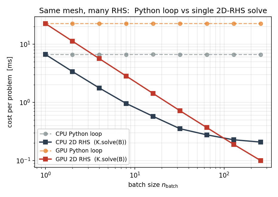
../_images/batched_rhs_scaling.png — Fig. 14 Per-problem cost on a 3014-node Poisson mesh: a Python loop that calls `tensormesh.sparse.SparseMatrix.solve()` `n_batch` times (dashed) versus a single 2D-RHS call (solid). On the GPU the speedup reaches `225x` at `n_batch = 256`.¶

The lesson reads cleanly off the figure. The loop is exactly n_batch independent solves, so each tick on the x-axis doubles its wall time. The 2D-RHS call factors K once and amortises that cost across every column; on the GPU it stays within \(\sim 15\%\) of the single-RHS time up to n_batch = 256.

Note

The factor-once amortisation is a property of the direct backends. If an iterative method runs instead – a very large GPU problem routes to native-PyTorch CG, or you pass method="cg" / "bicgstab" explicitly – torch-sla loops over the columns of a 2D RHS internally, so there is no factorisation to reuse and the only gain over a Python loop is reduced per-call dispatch overhead. torch-sla does not yet cache iterative-solver state (a preconditioner or Krylov basis reused across right-hand sides); a caching iterative solver is planned for a future release. See Sparse Solvers for how the backend and method are chosen.

Throughput is the same data the other way around – problems solved per second:

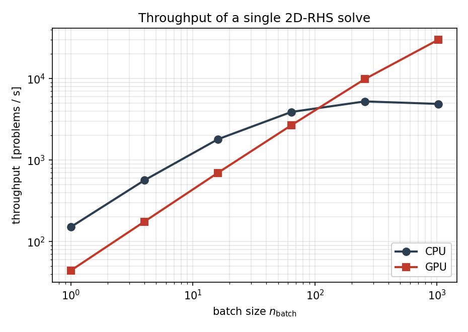
../_images/throughput.png — Fig. 15 Throughput in problems per second. The CPU path saturates the SuperLU back-substitution around \(5 \times 10^{3}\) problems per second; the GPU keeps climbing to nearly \(3 \times 10^{4}\) problems per second at `n_batch = 1024`.¶

Condensation works the same way. condense_rhs() accepts [n_dof, ...] shapes – the leading DOF axis is sliced and the trailing axes pass through:

condenser = Condenser(mesh.boundary_mask)
K_, _    = condenser(K, torch.zeros(mesh.n_points))
B_inner = condenser.condense_rhs(B)             # [n_inner, 64]
X_inner = K_.solve(B_inner)                     # [n_inner, 64]
X_full  = condenser.recover(X_inner)            # [n_dof, 64]

This is the workhorse pattern for ML training-data generation and for parametric studies where every problem shares the geometry.

Axis 3 – Multi-problem datasets¶

For ML workloads where you want many (input, output) pairs, tensormesh.dataset bundles two things:

MeshGen – programmatic Gmsh-backed mesh generation from CSG primitives (rectangles, circles, holes, …).
Multi-frequency equation classes that emit batched source terms with known analytical solutions, for supervised training:
- PoissonMultiFrequency (and …3D)
- HeatMultiFrequency
- WaveMultiFrequency
- LinearElasticityMultiFrequency (and …3D)

Each …MultiFrequency class samples random Fourier coefficients for the source term and – where applicable – returns the analytical solution at the same nodes, which is convenient for both training and validation.

The standard “same mesh, varying source” recipe combines this generator with the batched-RHS pattern from Axis 2:

import torch
from tensormesh import Mesh, LaplaceElementAssembler, MassElementAssembler, Condenser
from tensormesh.dataset import PoissonMultiFrequency

device = "cuda" if torch.cuda.is_available() else "cpu"

mesh      = Mesh.gen_rectangle(chara_length=0.02).to(device)
K         = LaplaceElementAssembler.from_mesh(mesh)().double()
M         = MassElementAssembler.from_mesh(mesh)().double()
condenser = Condenser(mesh.boundary_mask)
K_, _     = condenser(K, torch.zeros(mesh.n_points, device=device))

# 1024 random Poisson source terms, all evaluated at the same nodes.
eq = PoissonMultiFrequency(a=torch.rand(1024, 8, 8, device=device) * 2 - 1)
f  = eq.source_term(mesh.points, domain="rectangle").double()  # [1024, n_points]
b  = M @ f.T                                                   # [n_points, 1024]
b_ = condenser.condense_rhs(b)                                 # [n_inner, 1024]
u_ = K_.solve(b_)                                              # [n_inner, 1024]
u  = condenser.recover(u_)                                     # [n_points, 1024]

On a single RTX PRO 6000 the loop above produces 1024 Poisson solutions in roughly 34 ms (see the throughput figure above) – about \(30\,\mu\mathrm{s}\) per problem, dominated by the cuDSS triangular back-substitution. The fully benchmarked driver, with timing across many n_batch values, lives in examples/dataset/poisson/poisson_dataset.py.

For varying mesh workflows, regenerate Mesh per problem and pay the assembly cost each time – there is no shortcut for that case today.

What’s not built in¶

There is no built-in vmap-style assembler that vectorises K construction across many parameter values (e.g. one K per realisation of a stochastic coefficient field). For now two patterns work in user code:

Python loop – simplest, fine when assembly is cheap relative to solve.
``torch.vmap`` around the assembler call – works when the varying parameter enters via point_data or element_data and the result is uniform in shape. Note that vmap’s interaction with sparse output is fragile; test on small problems first.

A first-class batched-assembly API may show up in a future release; the dataset workflow above covers the most common case (same mesh, many sources) without it.

Reproducing the numbers¶

All three figures on this page come from a single script:

python docs/scripts/batched_workflows_figures.py

It uses only the public API and runs on CPU alone (the GPU panels are skipped on a CPU-only machine). On a CUDA host it writes batched_rhs_scaling.png, throughput.png, and memory_chunking.png into docs/source/_static/user_guide/batched_workflows/.

What’s next¶

Sparse Solvers – the backend / method auto-selection and the backend knobs that affect batched solves.
Differentiability – backprop through a batched pipeline.
Time Integration – transient problems where the inner solve at every time step is itself batched-RHS-shaped.