Taylor-Green Vortex (Convergence Study)
The Taylor-Green vortex is the canonical incompressible-flow
benchmark with a known exact solution: a periodic decaying vortex
on the square \([0, 2\pi]^2\) whose velocity and pressure can
be written down in closed form. The script
examples/fluid/taylor_green/taylor_green.py uses it to drive
a quantitative h-convergence study of the transient
Taylor-Hood Navier-Stokes solver — the only example in
Fluid Mechanics whose purpose is verification rather than
visualization.
Exact solution
For viscosity \(\nu\) and time \(t\),
The velocity decays exponentially with rate \(2\nu\) (twice the kinematic viscosity); the pressure decays at rate \(4\nu\). Substitution verifies that \((u, v, p)\) satisfies the incompressible Navier-Stokes equations exactly.
The script imposes Dirichlet velocities on every boundary node equal to the exact solution at the current time, and pins one pressure DOF to its exact value. This sidesteps the need for periodic boundaries and isolates the discretization error.
Solver
The transient NavierStokesTransientAssembler from
Cylinder Flow (Vortex Shedding) is reused verbatim — Taylor-Hood P2-P1 in
space (MixedElementAssembler), backward Euler
plus Picard sub-iterations in time, forward_vector for the
\(\rho/\Delta t\,\mathbf{u}^n\cdot\mathbf{v}\) load. The only
changes are:
domain \([0, 2\pi]^2\) (an order-2 generated mesh, so the P2 velocity nodes are the mesh points and the exact solution can be evaluated on them directly),
Dirichlet velocity from the exact solution rather than a parabolic inlet — updated each step via
condenser.update_dirichlet,\(L^2\) errors against the analytical velocity and pressure at the final time.
pin = layout.dof_index("p", int(layout.node_ids("p")[0]))

def dirichlet_values(t):
    bc_val = torch.zeros(layout.n_dofs, dtype=torch.float64)
    bc_val[layout.dof_mask("u")] = exact_velocity(points, t, nu).reshape(-1)
    bc_val[pin] = exact_pressure(x_p, t, nu)[0]
    return bc_val

for step in range(1, n_steps + 1):
    condenser.update_dirichlet(dirichlet_values(step * dt))
    u_prev = layout.split(sol)["u"]
    for _ in range(picard_iter):
        w = layout.split(u_iter)["u"]
        K = assembler(point_data={"w": w})
        f = assembler.assemble_vector(point_data={"uprev": u_prev})
        K_, f_ = condenser(K, f)
        u_iter = condenser.recover(K_.solve(f_))
    sol = u_iter
h-convergence
Taylor-Hood spatial theory promises \(\|\mathbf{u}_h - \mathbf{u}\|_{L^2} = \mathcal{O}(h^3)\) and \(\|p_h - p\|_{L^2} = \mathcal{O}(h^2)\) — but backward Euler contributes an \(\mathcal{O}(\Delta t)\) error on top. The study therefore couples \(\Delta t = h^2/4\), so the temporal error shrinks at least as fast as the \(\mathcal{O}(h^2)\) pressure error. In this slowly-decaying vortex (\(\nu = 0.01\)) the time-error constant is small, so the measured rates land at the spatial limits — \(\approx 3\) for the velocity, \(\approx 2\) for the P1 pressure:
Grid   h          L2_vel         L2_pres        Rate_vel   Rate_pres
----------------------------------------------------------------
10     0.6283     1.423434e-01   3.209651e-01   -          -
20     0.3142     1.862684e-02   8.626960e-02   2.93       1.90
40     0.1571     1.434308e-03   2.045441e-02   3.70       2.08
The plot taylor_green_convergence.png shows the same data on a
log-log axis with the reference \(h^2\) slope. If the observed
rates fall to 1, something in the solver is wrong — most often a
subtle bug in the boundary-condition imposition or the time
stepping.
Mass-weighted error norm
The script computes the discrete \(L^2\) norm via the mass matrix of the P2 space:
assembled by MassElementAssembler on the
order-2 mesh. The P1 pressure is prolonged into the P2 space first
(layout.prolong — exact, since \(P_1 \subset P_2\)), so
one mass matrix serves both fields. This is the right norm for FEM
error analysis, unlike the simple Euclidean norm of the nodal
error vector.
Output
Console table — convergence rates at every refinement step.
``taylor_green_convergence.png`` — log-log error plot vs mesh size with the reference slope.
``taylor_green_results.png`` — three-panel snapshot of the finest mesh: speed, pressure, velocity-error magnitude.
``taylor_green.mp4`` (optional) — animation of the decaying vortex.
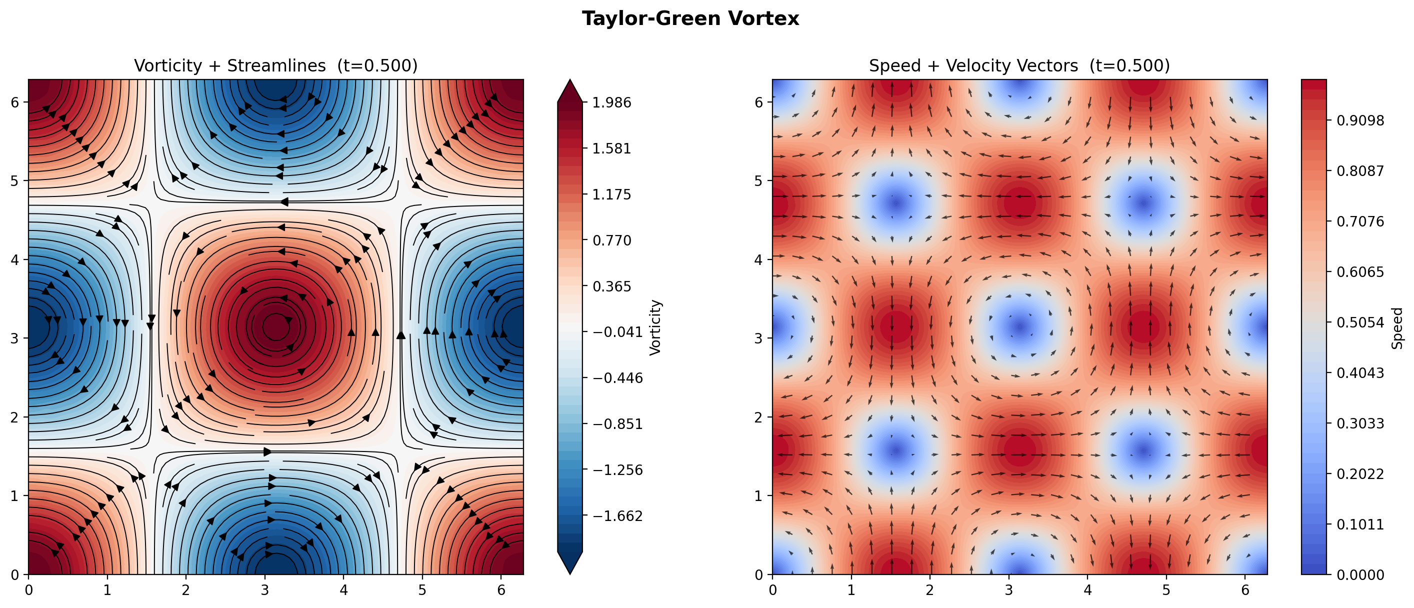
Fig. 71 Output of taylor_green.py at \(t=0.5\). Left: vorticity
field with overlaid streamlines — the canonical periodic
\(2\times2\) pattern of alternating-sign vortices. Right:
speed magnitude with velocity vectors, showing the characteristic
“saddle” structure between adjacent rolls. The amplitude has
decayed by \(\exp(-2\nu t)\) from the analytical initial
condition, which the script’s convergence study uses as
ground truth.
Running it
cd examples/fluid/taylor_green
python taylor_green.py      # writes convergence + results pngs
What’s next
Taylor-Hood Stokes — the steady counterpart: pure spatial convergence at the full Taylor-Hood rates.
Lid-Driven Cavity and Cylinder Flow (Vortex Shedding) — the qualitative NS solvers whose accuracy this example verifies.
Time Integration — a higher-order time integrator from
tensormesh.odewould expose the spatial \(h^3\) velocity rate.