Hyperelastic Beam (Neo-Hookean)

The simplest finite-strain example in the gallery: a \(1.0 \times 0.4 \times 0.4\) m rubber beam clamped at one end and twisted at the other by a torsional force field. Solved with a compressible Neo-Hookean strain-energy density and L-BFGS energy minimization. The script is examples/solid/hyperelastic_beam/hyperelastic_beam.py.

Why study this example before the harder ones below: it isolates the energy-minimization recipe on a clean geometry, with no holes, no contact, and no auxiliary fields — so what you see in the diff between this and cantilever_beam.py is exactly the move from “linear solve” to “L-BFGS over a nonconvex energy”.

Problem

Compressible Neo-Hookean strain energy:

\[\Psi(\mathbf{F}) \;=\; \frac{\mu}{2}\, (I_1 - 3) - \mu \ln J + \frac{\lambda}{2}\, (\ln J)^2,\]

where \(\mathbf{F} = \mathbf{I} + \nabla\mathbf{u}\) is the deformation gradient, \(I_1 = \mathrm{tr}(\mathbf{F}^T \mathbf{F})\), and \(J = \det\mathbf{F}\). The Lamé parameters \((\mu, \lambda)\) come from Rubber.lame_params in tensormesh.material (\(E \approx 10\) MPa, \(\nu \approx 0.48\), almost incompressible).

Boundary conditions:

• clamp at \(x = 0\): \(\mathbf{u} = \mathbf{0}\),

• torsional load at \(x = 1\): a Neumann traction \(\mathbf{t} = C\, (0, -z, y)\) with \(C = 2.4 \times 10^7\), integrated over the end facets with FacetAssembler to give a consistent nodal load \(f_i = \int_\Gamma N_i\, \mathbf{t}\, \mathrm{d}A\), ramped over 10 load steps,

• all other surfaces: traction-free.

TensorMesh setup

The NeoHookeanModel is a custom ElementAssembler whose element_energy returns \(\Psi(\mathbf{F})\) at each quadrature point — nothing more. TensorMesh integrates over elements, sums to a scalar total energy, and PyTorch’s autograd then provides the gradient for L-BFGS:

Listing 10 examples/solid/hyperelastic_beam/hyperelastic_beam.py (essence)

class NeoHookeanModel(ElementAssembler):
    def __post_init__(self, mu, lam):
        self.mu = mu
        self.lam = lam

    def element_energy(self, gradu):
        dim = gradu.shape[-1]
        I = torch.eye(dim, device=gradu.device, dtype=gradu.dtype)
        F = I + gradu
        J = torch.clamp(torch.det(F), min=1e-6)
        I1 = (F**2).sum()
        logJ = torch.log(J)
        return (0.5 * self.mu * (I1 - 3)
                - self.mu * logJ
                + 0.5 * self.lam * logJ**2)

mesh = gen_cube(chara_length=0.05, order=2,
                left=0, right=1.0, bottom=0, top=0.4,
                front=0, back=0.4)
model = NeoHookeanModel.from_mesh(mesh, mu=mu, lam=lam)

u = torch.zeros_like(mesh.points, requires_grad=True)
optimizer = optim.LBFGS([u], lr=1.0, max_iter=50,
                        history_size=50,
                        line_search_fn="strong_wolfe")

for step in range(1, n_load_steps + 1):
    lam_load = step / n_load_steps     # incremental load
    def closure():
        optimizer.zero_grad()
        u_active = apply_bcs(u, lam_load)
        E = model.energy(point_data={"displacement": u_active})
        E.backward()
        return E
    optimizer.step(closure)

A few details worth flagging:

• Quadratic tetrahedra (order=2). Linear (P1) tets lock in the near-incompressible limit (\(\nu \to 0.5\)). P2 elements are the cheapest fix for this problem.

• J-clamping. torch.clamp(J, min=1e-6) keeps the energy finite when L-BFGS overshoots into a folded configuration. A cleaner-but-slower alternative is to add a barrier term that pushes \(J\) back into \((0, \infty)\).

• Boundary conditions via masking. The script uses the pattern u_active = u * mask + val to enforce Dirichlet BCs inside the closure — gradients on masked DOFs are automatically zero, so L-BFGS leaves them alone. This avoids the need for a separate Condenser instance and works smoothly with autograd.

• Incremental loading is mandatory. Without it, L-BFGS warm-started from the rest configuration usually fails to find the basin at full torsion. 10 steps is enough for this beam; stiffer materials or more aggressive loading need more.

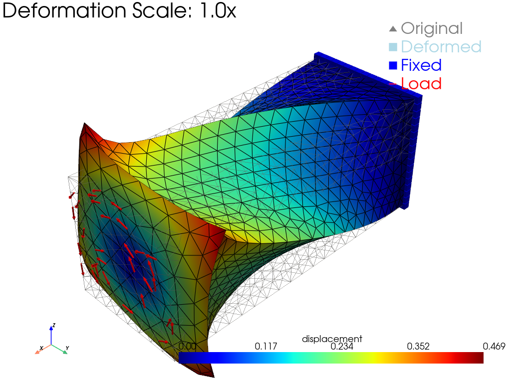
Fig. 43 Output of hyperelastic_beam.py: the rubber beam in its final twisted configuration, colored by displacement magnitude. The right end (blue cubes) is fixed; red arrows on the left end show the prescribed twisting load applied incrementally over 10 LBFGS load steps. Unlike the linear cantilever above, the deformation is shown at 1.0× — the Neo-Hookean response handles finite rotations without linearization artifacts.

Running it

cd examples/solid/hyperelastic_beam
python hyperelastic_beam.py     # writes hyperelastic_rubber.png

Console output reports the maximum nodal displacement at every load step.

What’s next

• Cantilever Beam — the linear-elastic counterpart; the diff between the two scripts is small but illuminating.

• Hertzian Contact — another L-BFGS-driven problem, this time with a contact-penalty energy.

• Forms — vector-valued element_energy returns and the autograd-based gradient.