Benchmark

This page compares TensorMesh against several established FEM frameworks on two forward problems (3D Poisson and 3D linear elasticity) and one inverse problem (compliance-minimization topology optimization).

All benchmark scripts and reference data live in a separate repository: camlab-ethz/tensormesh-bench.

Test environment

CPU	8 cores from a dual-socket AMD EPYC 9005-series (Zen 5 “Turin”) node
GPU	1× NVIDIA RTX PRO 6000 Blackwell Server Edition
Memory	64 GB DDR5 ECC (8 cores × 8 GB)
OS	Ubuntu 22.04 LTS (x86_64)

Compared frameworks

Framework	Backend	CPU	CUDA	Notes
FEniCS (DOLFINx)	C++/Python	✅	❌	8-rank MPI
Firedrake	Python/PETSc	✅	❌	8-rank MPI
MFEM	C++	✅	❌	8-rank MPI
scikit-fem	Python	✅	❌	Lightweight, single process
JAX-FEM	JAX	✅	✅	Differentiable
torch-fem	PyTorch	✅	✅	Differentiable
TensorMesh	PyTorch	✅	✅	Differentiable

Solver configuration

To keep the comparison controlled, every framework uses the same iterative linear solver and stopping criteria:

Parameter	Value
Iterative method	BiCGSTAB
Preconditioner	Jacobi (diagonal scaling)
Relative tolerance	\(10^{-10}\)
Absolute tolerance	\(10^{-10}\)
Maximum iterations	10,000

Note

The only exception is the CUDA path of torch-fem, which uses conjugate gradient (CG) instead of BiCGSTAB — its CUDA backend does not ship a BiCGSTAB implementation.

Forward problems

3D Poisson equation

On the unit cube \(\Omega = [0,1]^3\) we solve

\[\begin{split}\begin{cases} -\Delta u(\mathbf{x}) = f(\mathbf{x}) & \text{in } \Omega, \\ u(\mathbf{x}) = 0 & \text{on } \partial\Omega, \end{cases}\end{split}\]

with constant source \(f = 1\) and homogeneous Dirichlet boundary conditions on every face.

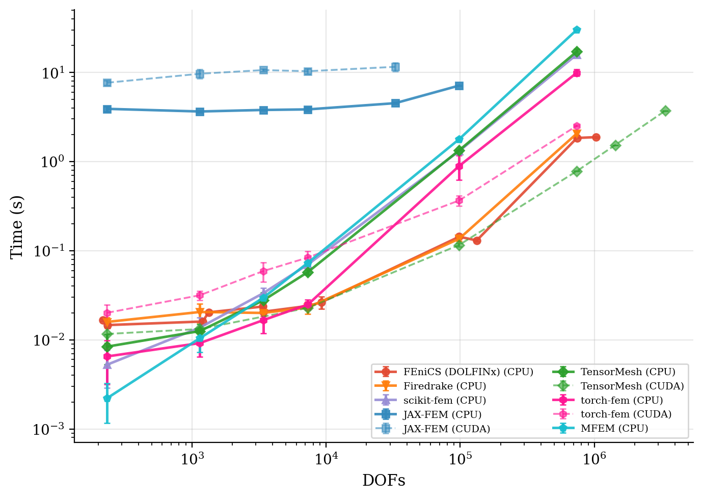
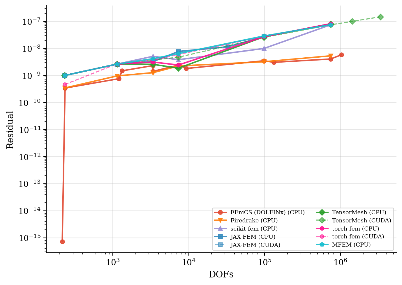
Solve time and residual convergence. Wall-clock time is plotted against problem size; residual histories show that every framework reaches the same target tolerance.

Solve time	Residual convergence

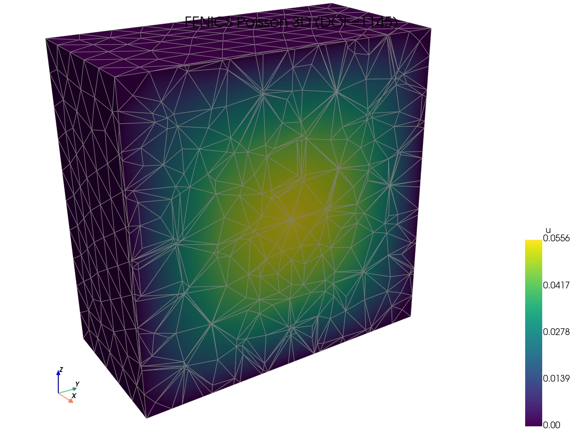
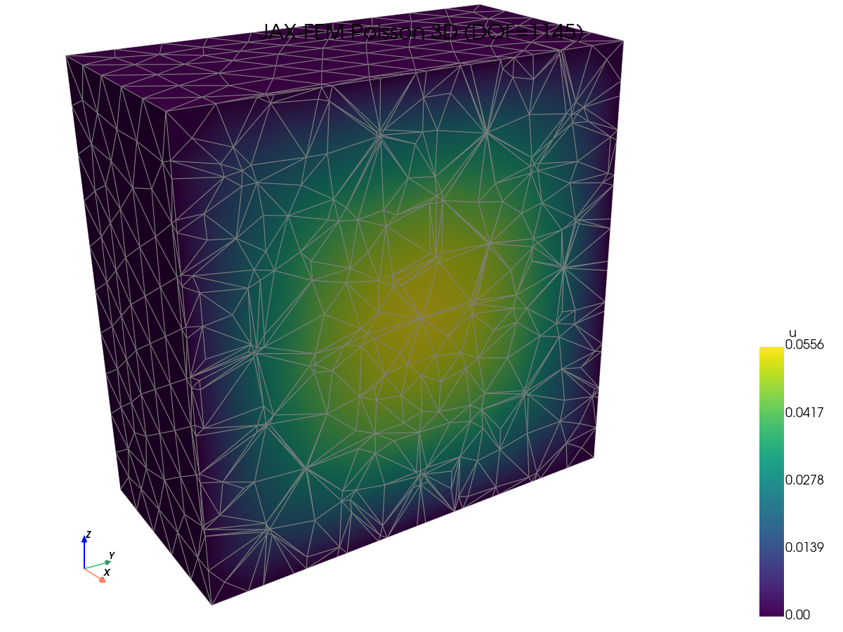
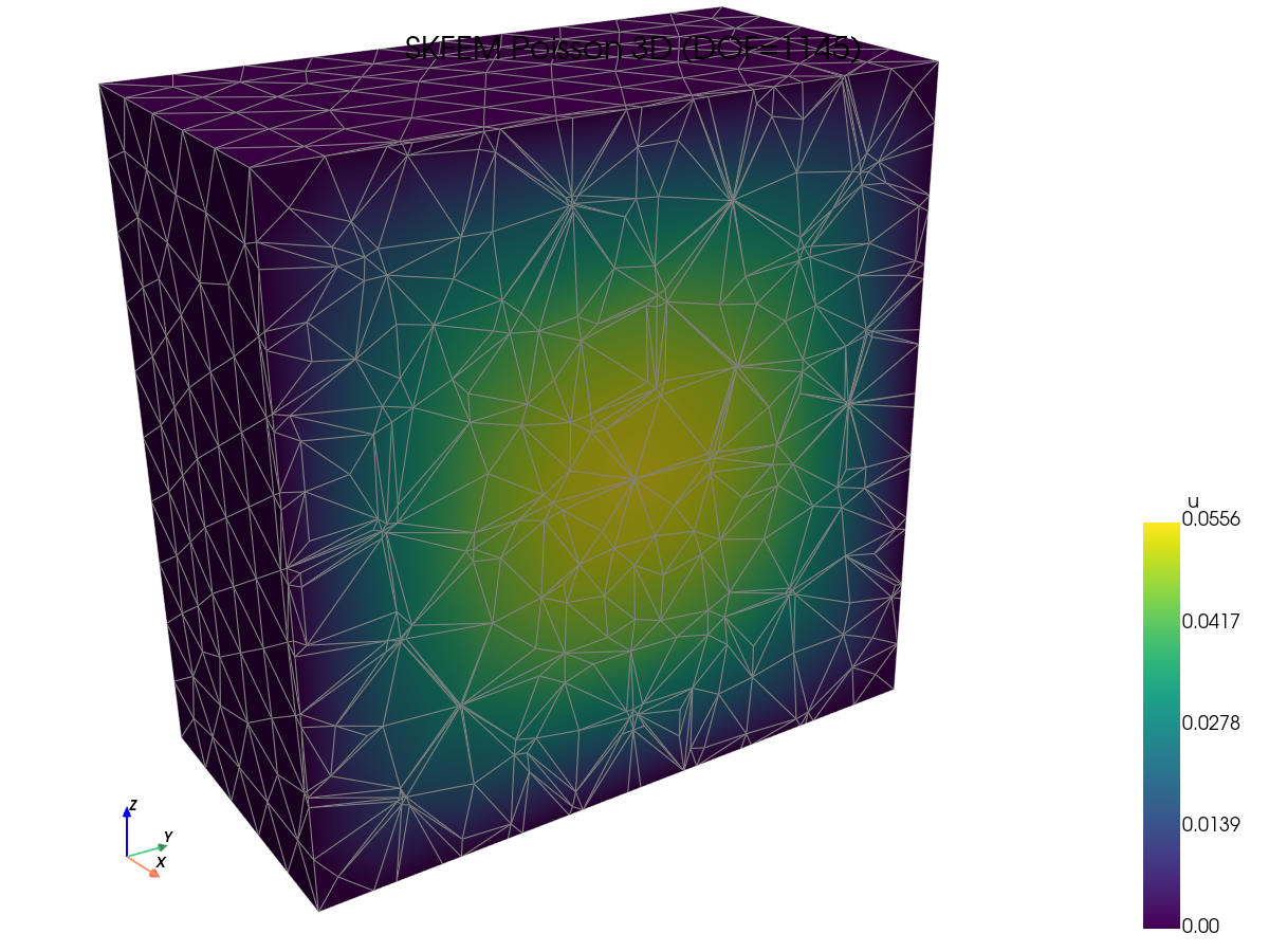
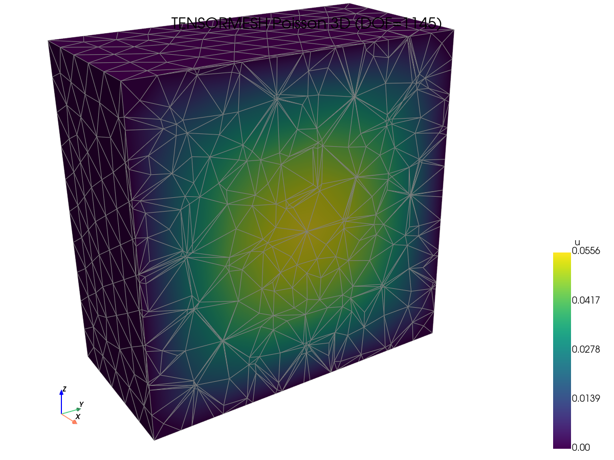
Solution visualizations. Spot-check that each framework produces the same field — useful as a sanity check before reading speed numbers.

FEniCS (DOLFINx)	JAX-FEM	scikit-fem	TensorMesh

3D linear elasticity

We solve the static equilibrium of an isotropic linear elastic body:

\[\begin{split}\begin{cases} -\nabla \cdot \boldsymbol{\sigma}(\mathbf{x}) = \mathbf{f}(\mathbf{x}) & \text{in } \Omega, \\ \mathbf{u}(\mathbf{x}) = \mathbf{0} & \text{on } \partial\Omega, \end{cases}\end{split}\]

where \(\mathbf{u} : \Omega \to \mathbb{R}^3\) is the displacement and the Cauchy stress satisfies Hooke’s law

\[\boldsymbol{\sigma} = \lambda \, \mathrm{tr}(\boldsymbol{\varepsilon}) \, \mathbf{I} + 2\mu \, \boldsymbol{\varepsilon}, \qquad \boldsymbol{\varepsilon} = \tfrac{1}{2}\bigl(\nabla \mathbf{u} + (\nabla \mathbf{u})^\top\bigr).\]

We set Young’s modulus \(E = 1\) and Poisson’s ratio \(\nu = 0.3\), giving

\[\lambda = \frac{E\nu}{(1+\nu)(1-2\nu)}, \qquad \mu = \frac{E}{2(1+\nu)}.\]

A constant body force \(\mathbf{f} = (1,1,1)^\top\) is applied. To introduce geometric complexity we use a hollow cube domain

\[\Omega = [0,1]^3 \setminus (0.25,\, 0.75)^3.\]

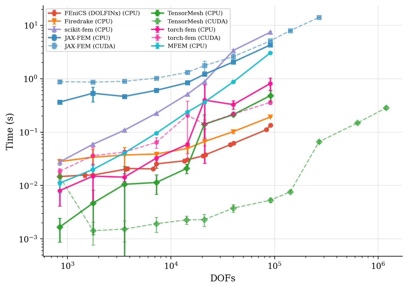
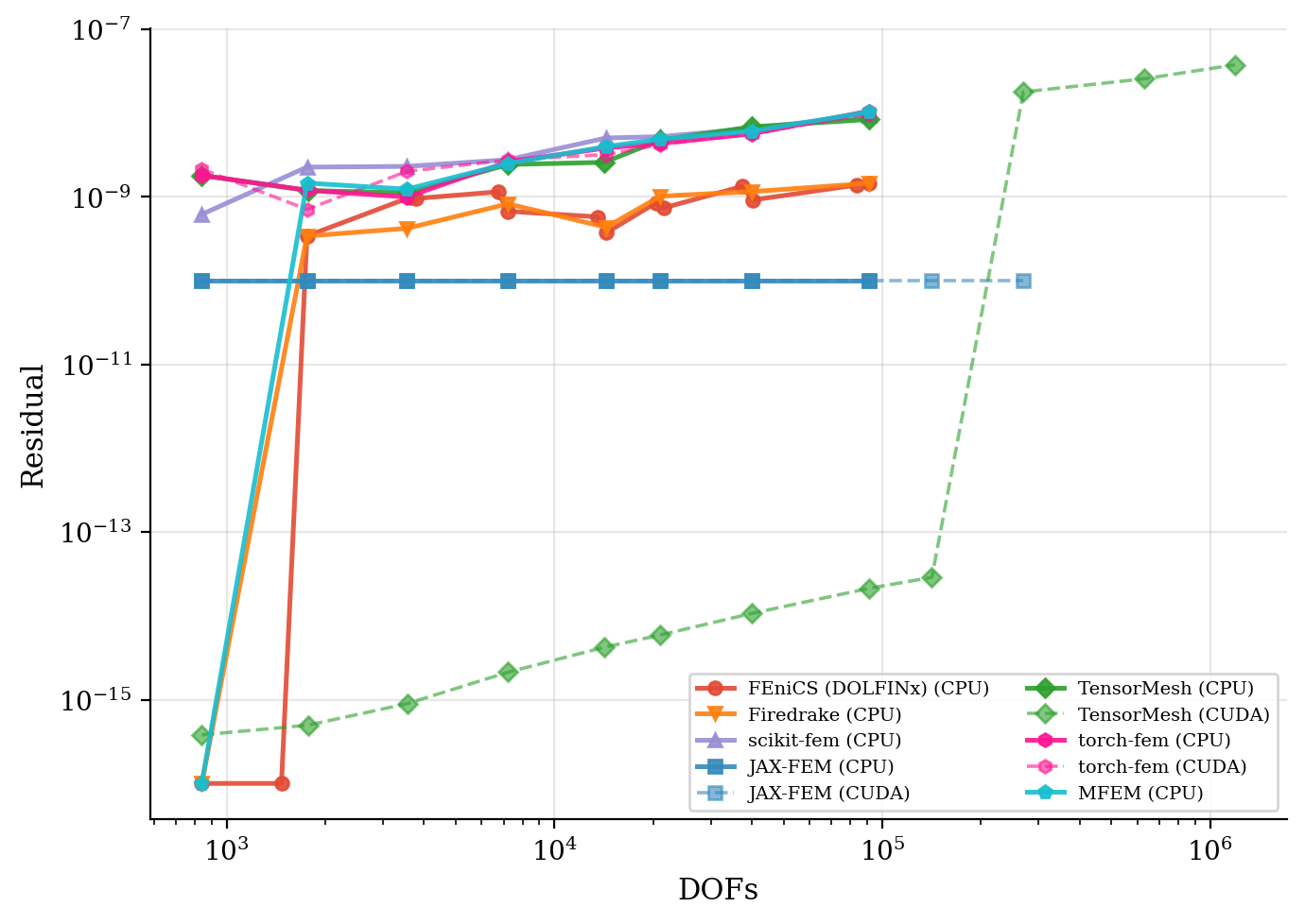
Solve time and residual convergence.

Solve time	Residual convergence

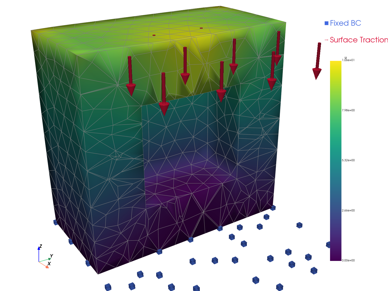
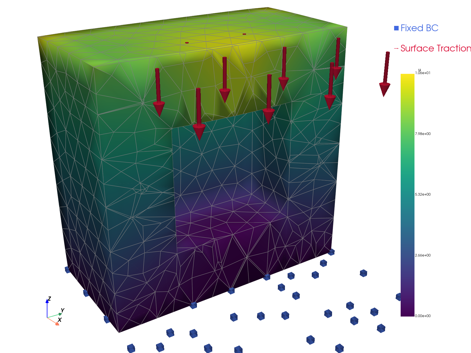
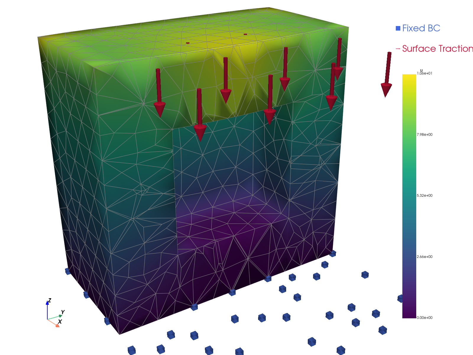
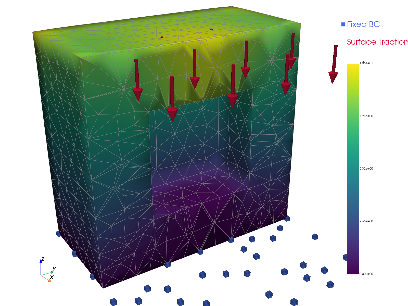
Solution visualizations.

FEniCS (DOLFINx)	JAX-FEM	scikit-fem	TensorMesh

Inverse problem: topology optimization

The inverse-problem benchmark exercises the differentiability of TensorMesh on a classical topology-optimization task: compliance minimization of a 2D cantilever beam using the Solid Isotropic Material with Penalization (SIMP) method. We compare against JAX-FEM, the only other framework in the list above that supports end-to-end automatic differentiation through the FEM pipeline.

Problem setup

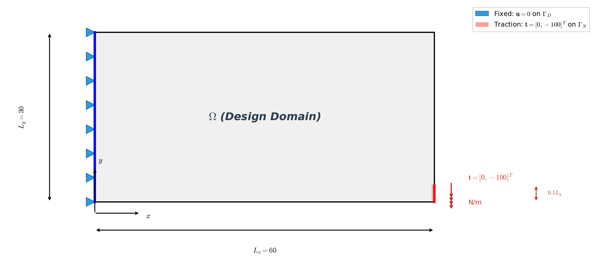
The computational domain is a rectangle \(\Omega = [0, L_x] \times [0, L_y]\) with \(L_x = 60\) and \(L_y = 30\) (dimensionless), discretized into \(60 \times 30\) bilinear quadrilateral (QUAD4) elements — 1,891 nodes and 1,800 elements. Homogeneous Dirichlet conditions are imposed on the left edge,

\[\mathbf{u} = \mathbf{0} \quad \text{on } \Gamma_D = \{(x,y) : x = 0\},\]

and a distributed traction is applied to the lower portion of the right boundary,

\[\mathbf{t} = (0,\, -100)^\top \;\text{N/m} \quad \text{on } \Gamma_N = \{(x,y) : x = L_x,\; 0 \leq y \leq 0.1\, L_y\}.\]

The element stiffness is parameterized by the SIMP interpolation

\[E(\rho) = E_{\min} + \rho^p \,(E_{\max} - E_{\min}),\]

where \(\rho \in [\rho_{\min}, 1]\) is the element-wise density (the design variable), \(p = 3\) penalizes intermediate densities, \(E_{\max} = 70{,}000\) MPa is the solid stiffness, and \(E_{\min} = 70\) MPa keeps the stiffness matrix non-singular. The Poisson’s ratio is \(\nu = 0.3\).

The optimization minimizes structural compliance subject to a volume constraint:

\[\begin{split}\begin{aligned} \min_{\boldsymbol{\rho}} \quad & C(\boldsymbol{\rho}) = \mathbf{u}^\top \mathbf{K}(\boldsymbol{\rho}) \mathbf{u} = \mathbf{F}^\top \mathbf{u} \\ \text{s.t.} \quad & \frac{1}{|\Omega|} \int_{\Omega} \rho \, d\Omega \leq \bar{v} \\ & \mathbf{K}(\boldsymbol{\rho}) \mathbf{u} = \mathbf{F} \\ & \rho_{\min} \leq \rho_e \leq 1, \quad \forall e \end{aligned}\end{split}\]

with target volume fraction \(\bar{v} = 0.5\) and \(\rho_{\min} = 10^{-3}\). We use the Method of Moving Asymptotes (MMA) with move limit \(\Delta\rho_{\max} = 0.1\) and a sensitivity filter of radius \(r_{\min} = 1.5\,h\) (where \(h\) is the element size) to suppress checkerboard patterns. The optimization runs for 51 iterations.

Sensitivity via automatic differentiation

The classical adjoint-method sensitivity for SIMP has the closed form

\[\frac{\partial C}{\partial \rho_e} = -p\, \rho_e^{p-1} (E_{\max} - E_{\min})\, \mathbf{u}_e^\top \mathbf{K}_0^e \mathbf{u}_e,\]

where \(\mathbf{K}_0^e\) is the element stiffness at unit Young’s modulus. In TensorMesh this gradient is not implemented manually — it is obtained by backpropagating through the differentiable assembly and sparse solve via PyTorch’s reverse-mode autograd. The closed-form expression above is reproduced only for reference and as a consistency check against the autograd output.

Final design comparison

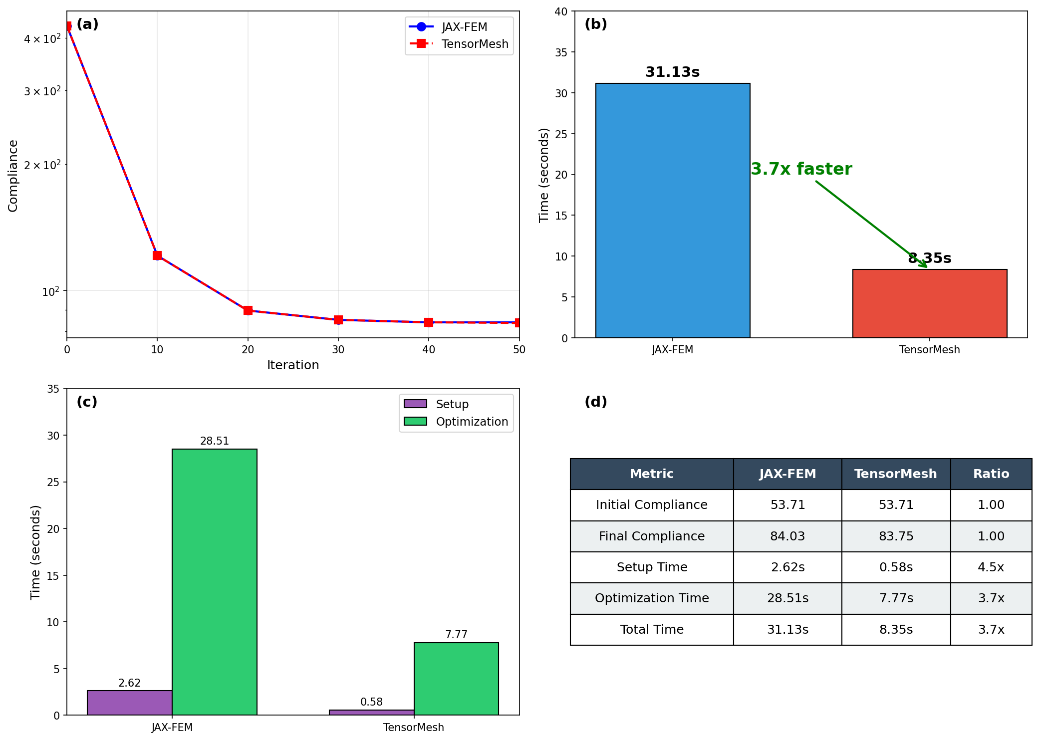
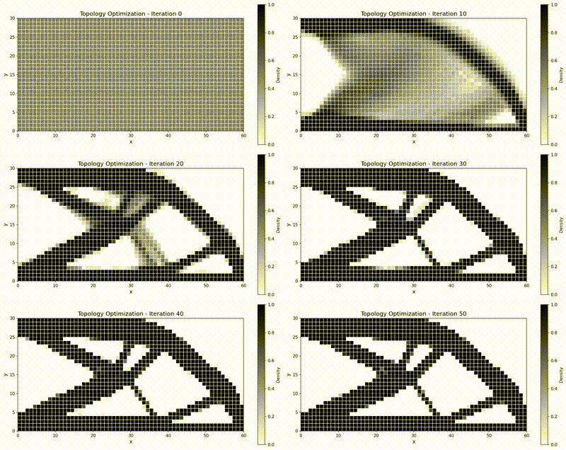
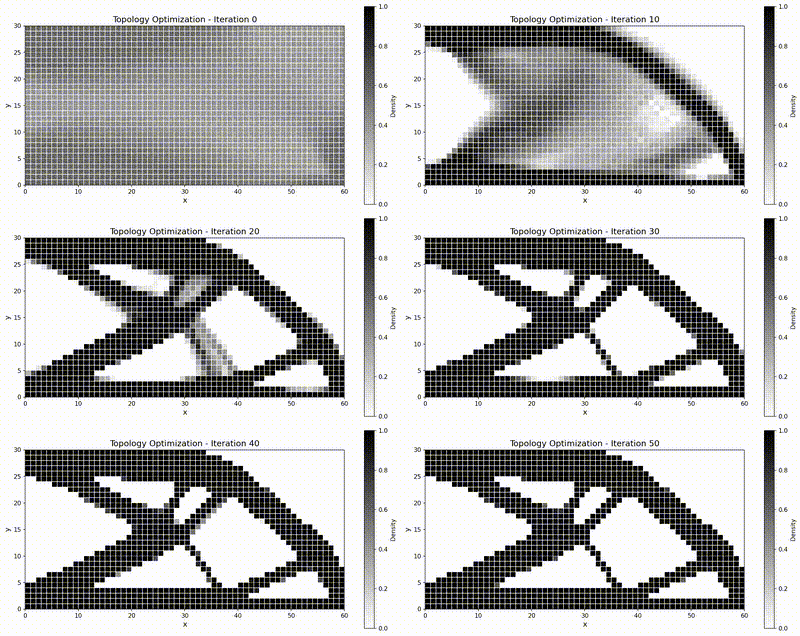
Both frameworks converge to the same canonical truss-like topology, and TensorMesh runs noticeably faster end-to-end thanks to GPU-resident assembly and solve.

Optimization animations

JAX-FEM	TensorMesh