Flow Past Multiple Obstacles

A steady Navier-Stokes example that highlights TensorMesh’s
mesh-generation capabilities as much as its FEM machinery. The
script examples/fluid/flow_obstacles/flow_obstacles.py solves
incompressible flow at \(\mathrm{Re} = 150\) through a
\(3 \times 1\) channel containing six circular obstacles of
varying size and position. The mesh is generated programmatically
via MeshGen using CSG (constructive solid
geometry): start with a rectangle, subtract six discs.
The discretization is the same Taylor-Hood P2-P1 mixed pair as
Lid-Driven Cavity — and like Cylinder Flow (Vortex Shedding), the MeshGen mesh is
linear, so the quadratic velocity space is generated
topologically on top of it by the
MixedElementAssembler.
Problem
with the channel \((0, 3) \times (0, 1)\) minus six discs at
Boundary conditions:
inlet (\(x = 0\)): parabolic profile, \(u_x(y) = 4\,y\,(1 - y)\),
walls (\(y = 0\), \(y = 1\)) and obstacle surfaces: no-slip,
outlet (\(x = 3\)): “do-nothing” (natural), which also fixes the pressure gauge — no pressure BC at all.
At \(\mathrm{Re} = 150\) the flow is steady (no shedding), the wake of each obstacle interacts with the next, and the solution shows characteristic narrow jets between the closely- spaced cylinders.
Mesh generation via CSG
The most interesting part of this script is the mesh-generation
block — it is short, self-contained, and demonstrates the
add_… / remove_… style of CSG that
MeshGen exposes:
from tensormesh import MeshGen

gen = MeshGen(chara_length=1.0/n_grid)
gen.add_rectangle(0, 0, 3.0, 1.0)
for ox, oy, orad in [
    (0.5, 0.5, 0.10), (1.0, 0.3, 0.08), (1.0, 0.7, 0.08),
    (1.5, 0.5, 0.12), (2.0, 0.4, 0.07), (2.0, 0.6, 0.07),
]:
    gen.remove_circle(ox, oy, orad)
mesh = gen.gen().double()
Under the hood, MeshGen defers to Gmsh’s OpenCASCADE backend
for the boolean operations and triangulation, then converts back
into a Mesh with its internal element
ordering. See Meshes for the full
MeshGen API.
Solver
Identical to Lid-Driven Cavity — the same two-field
NavierStokesAssembler (Picard-linearized convection, four-line
scalar integrand) with richer boundary masks. Because the velocity
DOFs include topologically generated edge nodes, the masks are
built from the layout’s own coordinates and boundary detection —
no geometric distance tests against the obstacle circles needed:
x_u = layout.points("u")                                # P2 node coords
is_boundary = layout.split(layout.boundary_mask("u"))["u"][:, 0]
is_inlet = is_boundary & (x_u[:, 0] < eps)
is_outlet = x_u[:, 0] > LENGTH - eps
no_slip = is_boundary & ~is_inlet & ~is_outlet          # walls + obstacles

bc_mask = layout.dof_mask("u", node_mask=is_inlet | no_slip)
y_in = x_u[is_inlet, 1]
bc_val[layout.dof_mask("u", node_mask=is_inlet, component=0)] = \
    4.0 * y_in * (1.0 - y_in)

# Picard loop: lagged velocity on the P2 field's own DOFs
K = assembler(field_data={"w": ("u", w)})
The obstacle surfaces fall out of the topological classification automatically: they are boundary nodes that are neither inlet nor outlet.
Output
flow_obstacles.png is the final figure: speed magnitude and
pressure contour overlaid on the obstacle silhouettes. Useful
sanity checks on the picture:
a high-speed jet between the two upper-row obstacles at \(x \approx 1.0\),
a broad recirculation zone behind the largest obstacle at \((1.5, 0.5)\),
near-uniform pressure drop across the channel.
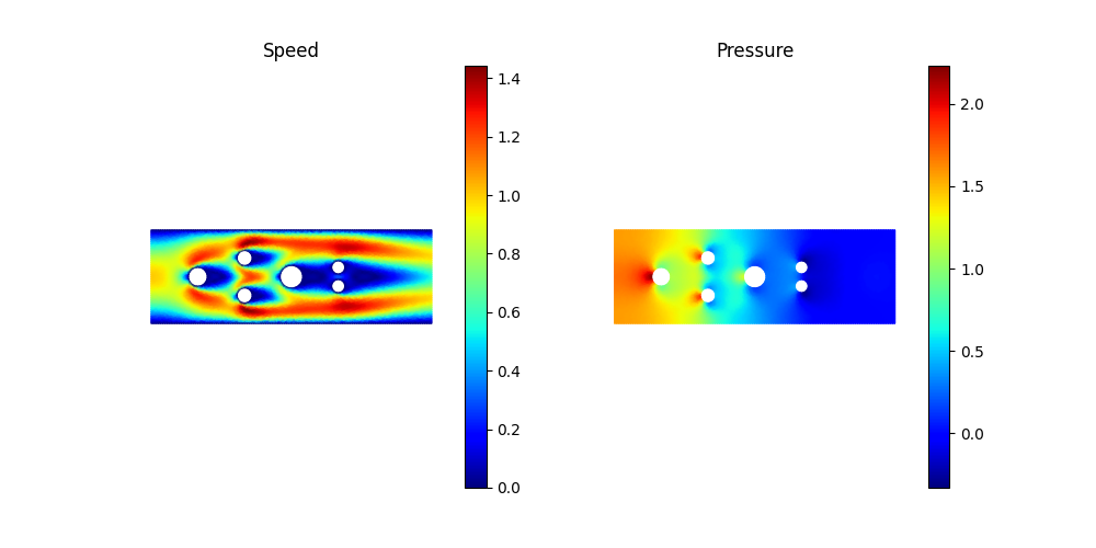
Fig. 69 Output of flow_obstacles.py at Re = 150 (Taylor-Hood P2-P1).
Left: speed magnitude — high-velocity jets squeeze between
obstacle pairs and broaden into wakes downstream. Right:
pressure — stagnation upstream of each obstacle, low-pressure
pockets in the wakes, and a near-uniform streamwise pressure
drop across the channel.
Running it
cd examples/fluid/flow_obstacles
python flow_obstacles.py     # writes flow_obstacles.png
At the default resolution (51k DOFs) the Picard loop converges in 8 iterations.
What’s next
Lid-Driven Cavity — the simpler steady benchmark.
Cylinder Flow (Vortex Shedding) — the transient version of “flow past a body”, where shedding takes over.
Meshes — full
MeshGenAPI including 3D primitives and hybrid meshes.Mixed Assembly — topological P2 spaces on linear meshes (generalized order pairs).