Distributed FEM

Three scripts in examples/distributed/ cover the building blocks for multi-GPU FEM in TensorMesh: graph coloring on the element adjacency graph, spectral domain decomposition, and a single-GPU-vs-multi-GPU assembly benchmark on a structured tetrahedral cube.

Caution

The distributed layer is still under active development. The building blocks below (coloring, partitioning, multi-GPU assembly) work and the benchmarks are real, but the public API is not yet stable and the User Guide deliberately does not document it as a first-class workflow. The next step is to couple it with torch-sla’s distributed linear solver, so that assembly and solve both run across multiple GPUs — the goal being to tackle very large-scale industrial problems that do not fit on a single device. Until then, treat the examples here as recipes to learn from, not as a stable interface.

Element-graph coloring — graph_coloring.py

Race-free atomic-add assembly on GPU needs a coloring of the element-adjacency graph: elements that touch a common DOF must not share a color, so each color class can be scattered into the global matrix in parallel. mesh.color() does this in one call, running a parallel Welsh-Powell-style heuristic on the GPU when available:

Listing 23 examples/distributed/graph_coloring.py (essence)

from tensormesh.dataset.mesh import gen_rectangle

mesh = gen_rectangle(chara_length=1.0/50, element_type="tri")
mesh.to(device)

colors = mesh.color()                    # one int per element
n_colors = colors.max().item() + 1
print(f"Used {n_colors} colors.")

For a regular triangulation of the unit square the algorithm typically finds 6–8 colors — close to the optimal chromatic number for a 2D triangle adjacency graph. The visualization paints each element by its color class, which gives the familiar striped / banded pattern.

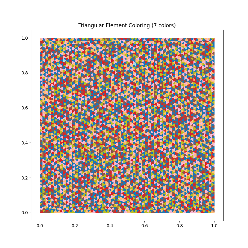
Fig. 58 graph_coloring.py output: a triangular mesh of the unit square painted by element color class. The Welsh-Powell heuristic finds 7 colors here; elements sharing a color never share a node, so each color class can be assembled in parallel without write conflicts.

Spectral domain decomposition — graph_partition.py

For multi-GPU work the mesh has to be split into n_parts balanced subdomains with small interfaces. partition_mesh with method="spectral" computes the Fiedler vector of the graph Laplacian and recursively bisects:

Listing 24 examples/distributed/graph_partition.py (essence)

from tensormesh.mesh.partition import partition_mesh

submeshes = partition_mesh(mesh, n_parts=4, method="spectral")

The returned list of Mesh objects each carries ghost nodes — the boundary nodes that belong to two subdomains get duplicated, with their original global IDs stored in submesh.point_data["orig_nid"]. The script’s exploded-view visualization separates the four subdomains in space and circles the shared interface nodes — the geometric picture you usually have to draw on a whiteboard to explain a domain decomposition.

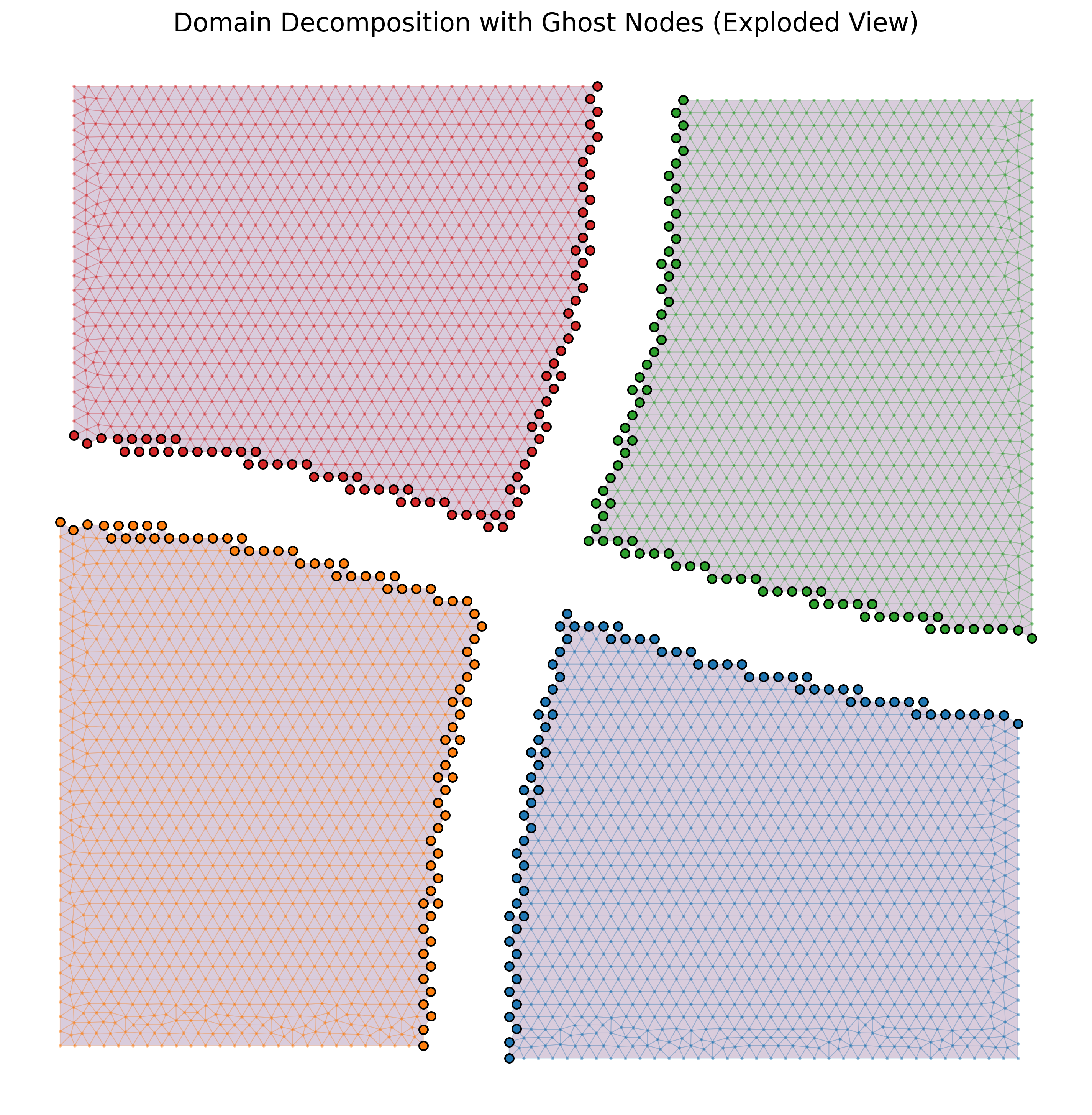
Fig. 59 graph_partition.py output: a 4-way spectral partition of the unit square in exploded view. Each subdomain is rendered in its own color; the highlighted dots along each subdomain’s shared boundary are the ghost nodes — duplicated copies of the interface vertices that each rank owns locally, with the original global IDs preserved in submesh.point_data["orig_nid"].

Multi-GPU assembly benchmark — benchmark_assembly.py

The headline distributed-FEM benchmark. A structured tetrahedral cube of size \((n+1)^3\) points and \(5 n^3\) tets is assembled (i) on a single GPU, (ii) across all visible GPUs via torch.multiprocessing. The driver sweeps \(n\) from a configurable starting size until either path runs out of memory.

The interesting machinery lives in DistributedMesh, which wraps the spectral partition + per-subdomain ghost-node bookkeeping into a single object:

Listing 25 examples/distributed/benchmark_assembly.py (essence)

import torch.multiprocessing as mp
from tensormesh.distributed import DistributedMesh

def _mp_assemble_worker(rank, submesh, device_id, q_order, return_dict):
    device = torch.device(f"cuda:{device_id}")
    torch.cuda.set_device(device)
    submesh.to(device)
    asm = tm.LaplaceElementAssembler.from_mesh(
        submesh, quadrature_order=q_order
    )
    K_local = asm()
    # …translate K_local.row/col through orig_nid into global indices…

dmesh = DistributedMesh(mesh, num_partitions=num_partitions)
manager = mp.Manager(); return_dict = manager.dict()
procs = [
    mp.Process(target=_mp_assemble_worker,
               args=(i, dmesh.submeshes[i], i, q_order, return_dict))
    for i in range(num_partitions)
]
for p in procs: p.start()
for p in procs: p.join()

A few details that matter:

• One process per GPU. torch.multiprocessing with set_start_method("spawn") gives each process its own Python interpreter, sidestepping the GIL. Threading would not help on CPU-bound assembly.

• Ghost-node bookkeeping. Each worker assembles a local SparseMatrix whose row/col are local DOF indices; the driver translates them through orig_nid into global indices before stitching the partial matrices together. The user-visible cost is a single GPU→CPU copy per worker.

• Per-card memory. The benchmark’s “mem save” column reports single_gpu_peak / max_per_card_peak — typically close to num_partitions for the assembly step itself, since each worker only stores its own subdomain.

A representative slice of the output table:

    n |   Points |    Tets | 1-GPU time | 1-GPU mem | N-GPU wall  N-GPU max_t  N-GPU mem/card | Speedup  Mem save
----------------------------------------------------------------------------------------------------------------
   30 |   29,791 | 135,000 |    0.42 s  |    0.5 GB |     0.18 s     0.11 s         0.16 GB  |    2.3x      3.1x
   50 |  132,651 | 625,000 |    1.90 s  |    2.3 GB |     0.55 s     0.34 s         0.62 GB  |    3.5x      3.7x
   …   …          …          …            …            …            …               …          …          …

CLI:

python benchmark_assembly.py                          # auto-detect GPUs
python benchmark_assembly.py --partitions 4 --start 30 --max 200

Running the examples

cd examples/distributed
python graph_coloring.py        # writes graph_coloring_result.png
python graph_partition.py       # writes graph_partition_exploded.png
python benchmark_assembly.py    # prints benchmark table

All three are lightweight and run on a single workstation; only benchmark_assembly.py benefits from multiple GPUs.

What’s next

• Concepts — the module map mentions tensormesh.distributed as a research path.

• Batched Workflows — single-GPU batching patterns that often suffice before reaching for multi-GPU.

• Basics & Visualization — plot_mesh.py has the adjacency-graph visualizations these algorithms operate on.