Meshes

A Mesh is the geometric and topological foundation of every problem in TensorMesh. It holds the points, the connectivity of one or more element types, and any per-node or per-element data attached to them. Because Mesh extends torch.nn.Module, you move it to a device with mesh.to("cuda"), serialize it with state_dict, and let autograd track gradients through anything that touches its tensors.

The Mesh data structure

Every mesh exposes the same six attributes:

Attribute	Type	Shape / contents
points	torch.Tensor	[n_points, dim] — coordinates of every DOF / interpolation node (= every degree of freedom of a scalar field). For order=1 this is the same as the element vertices; for order ≥ 2 it also includes mid-edge, mid-face, and interior nodes.
cells	BufferDict[str, torch.Tensor]	keyed by element type (e.g. "triangle", "hexahedron27"); each value is [n_elements, n_basis] long-integer connectivity.
point_data	BufferDict[str, torch.Tensor]	per-node fields. Keys starting with is_ or ending in _mask are auto-cast to bool on load (e.g. is_boundary).
cell_data	ModuleDict[str, BufferDict[str, torch.Tensor]]	per-element fields, nested by element type then field name.
field_data	BufferDict[str, torch.Tensor]	mesh-global metadata (rare).
cell_sets	dict	meshio-style named subsets, kept opaque on round-trip.

Because cells is a dict, mixed-element meshes (triangles + quads, tets + hexes, …) are first-class. Iterating mesh.cells.items() gives you each element block in turn.

Useful properties: mesh.n_points, mesh.n_elements, mesh.dim (= mesh.points.shape[1]), mesh.dtype, mesh.device, and mesh.default_element_type (the highest-dimensional type, falling back to a list for mixed meshes).

Note

Throughout this guide and the API, “point” means DOF / interpolation node, not “corner vertex of an element”. The two coincide for linear elements but diverge for higher orders: a Mesh.gen_rectangle(chara_length=0.3, order=2) carries 101 points against only 30 corner vertices — the 71 extras are the mid-edge nodes of the triangle6 cells. The shape of points therefore also matches the length of any 1-D field you put into point_data.

Built-in generators

For domains with simple shapes, TensorMesh ships a Gmsh-backed generator family. All return a Mesh ready to use and accept chara_length (target element size) and order (polynomial order) as the two universal knobs:

Generator	Default element	Domain
gen_rectangle()	"tri"	axis-aligned rectangle on [left, right] × [bottom, top]
gen_hollow_rectangle()	"quad"	rectangle with rectangular hole
gen_circle()	"tri"	disk of radius r centered at (cx, cy)
gen_hollow_circle()	"quad"	annulus
gen_L()	"quad"	L-shaped 2D domain
gen_cube()	"tet"	axis-aligned 3D box
gen_hollow_cube()	"tet"	cube with cubic hole
gen_sphere()	"tet"	solid ball of radius r
gen_hollow_sphere()	"tet"	spherical shell

A typical call and the resulting mesh:

from tensormesh import Mesh

mesh = Mesh.gen_rectangle(chara_length=0.1)
print(mesh)

Mesh(
    points: torch.Size([144, 2])
    cells: line:torch.Size([40, 2]),triangle:torch.Size([246, 3])
    point_data: is_boundary(torch.bool):144,is_left_boundary(torch.bool):144,is_right_boundary(torch.bool):144,is_bottom_boundary(torch.bool):144,is_top_boundary(torch.bool):144,gmsh:dim_tags(torch.int64):2
    cell_data: gmsh:physical(torch.int64):40,gmsh:geometrical(torch.int64):40
    field_data: boundary(torch.int64):2,domain(torch.int64):2
)

Notice three things in the real output that the table above does not hint at:

• cells contains a line block alongside triangle — the generators retain the 1-D boundary facets so that FacetAssembler can integrate over them directly.

• point_data already carries per-side boundary masks (is_left_boundary, is_right_boundary, …) in addition to the union is_boundary. You get region-aware Dirichlet BCs for free.

• The gmsh:* keys and field_data are the underlying Gmsh physical-group metadata, preserved on round-trip but rarely needed in user code.

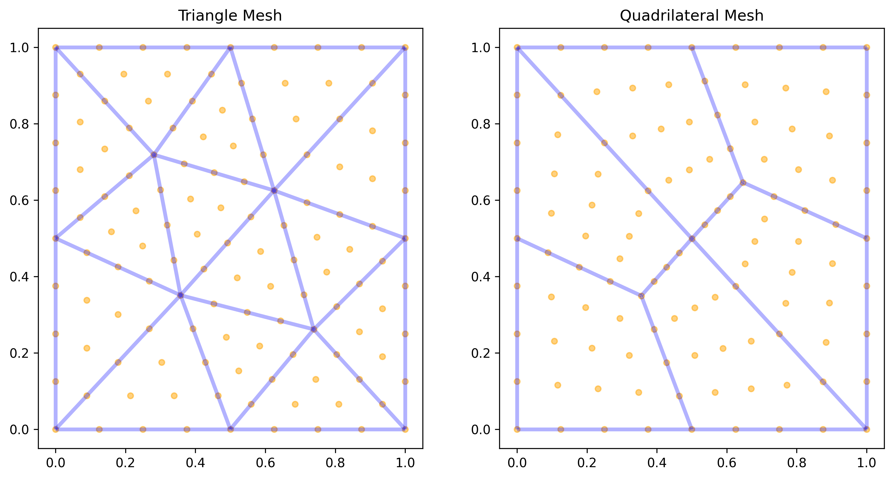
Fig. 1 gen_rectangle() produces a tri (left) or quad (right) mesh of the rectangle. Mid-edge nodes (orange) are visible because this figure uses order=2; with order=1 only the corner vertices remain.

Smaller chara_length → finer mesh (and finer means quadratically more points in 2D, cubically in 3D). Use order=2 to get triangle6 / quad9 / tetra10 / hexahedron27 instead of the linear default.

Composing custom geometries with MeshGen

When the shape you need is not one of the built-ins but is still expressible as a Boolean combination of primitives — a plate with holes, a domain with mixed element types, a 3-D part with cavities — reach for MeshGen instead of writing a .geo file by hand. It is a thin, scriptable wrapper around the Gmsh OCC kernel that returns a TensorMesh Mesh directly:

import tensormesh as tm

gen = tm.MeshGen(element_type=None, chara_length=0.1, order=2)
gen.add_rectangle(0,   0, 0.5, 1, element="tri")    # left half: triangles
gen.add_rectangle(0.5, 0, 0.5, 1, element="quad")   # right half: quads
gen.remove_circle(0.5, 0.5, 0.1)                    # punch a hole
mesh = gen.gen()

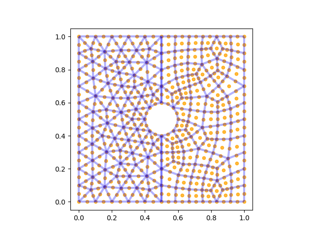
Fig. 2 The mesh produced by the snippet above — order-2 triangles on the left, order-2 quadrilaterals on the right, fused along a shared interface, with a circular hole punched out. Orange dots are the interpolation nodes (mid-edge nodes are present because order=2).

The same API extends to 3-D (dimension=3 plus add_cube / remove_sphere), and element_type=None enables hybrid meshes where different regions use different element types — fully supported downstream because cells is a dict keyed by element type.

A picture catalogue of what MeshGen and the built-in generators can produce — primitives, hybrid meshes, adjacency overlays, field visualizations — lives in the Mesh generation gallery of the example gallery.

For geometries that go beyond CSG (CAD imports, named physical boundaries, anisotropic sizing fields), drive Gmsh directly and load the result via meshio (see I/O — loading and saving below).

Per-node and per-element data

Attach a field to every node:

import torch
u = torch.zeros(mesh.n_points)
mesh.register_point_data("u", u)            # appears in mesh.point_data
print(mesh.point_data["u"].shape)            # torch.Size([144])

The chained form mesh.register_point_data(...) returns the mesh, which is convenient when building up a result before saving.

Per-element fields work the same way, keyed by element type:

energy = torch.zeros(mesh.n_elements)
mesh.register_element_data("strain_energy", energy)
# Equivalent to mesh.cell_data["triangle"]["strain_energy"] = energy

The lower-level cells, point_data, cell_data are full BufferDict objects — you can read them with [...], iterate them, or move them with .to(device).

Boundary identification

The generators all populate point_data["is_boundary"] (a bool tensor over points), which the convenience property exposes as:

mesh.boundary_mask        # bool tensor, shape [n_points]
mesh.boundary_mask.sum()  # number of boundary nodes

Hand-rolled meshes can use either is_boundary or boundary_mask as the key — the property accepts both.

Per-side masks come for free. The 2-D / 3-D rectangular and cuboidal generators (gen_rectangle(), gen_hollow_rectangle(), gen_L(), gen_cube(), …) also register one is_<side>_boundary mask per face so you can pin Dirichlet values on a single edge or face without recomputing the geometry:

mesh = tm.Mesh.gen_rectangle(chara_length=0.1)
list(k for k in mesh.point_data.keys() if k.endswith("_boundary"))
# ['is_boundary', 'is_left_boundary', 'is_right_boundary',
#  'is_bottom_boundary', 'is_top_boundary']

int(mesh.point_data["is_left_boundary"].sum())   # 11

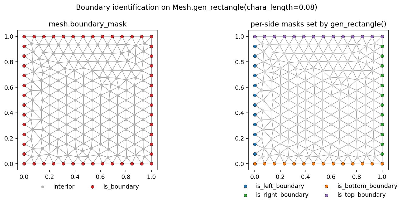
Fig. 3 Boundary points on Mesh.gen_rectangle(chara_length=0.08). Left: the union mask mesh.boundary_mask. Right: the four per-side masks set automatically by the generator, ready to feed into a region-aware Condenser.

For curved domains (gen_circle(), gen_sphere(), …) or hand-rolled meshes, derive your own masks from coordinates and store them as additional point_data entries:

x, y = mesh.points[:, 0], mesh.points[:, 1]
left   = (x == 0)
right  = (x == 1)
mesh.register_point_data("left_mask",  left)
mesh.register_point_data("right_mask", right)

These plug straight into a Condenser for non-homogeneous Dirichlet BCs (see Boundary Conditions).

I/O — loading and saving

TensorMesh round-trips through meshio, so any format meshio understands (.msh, .vtk, .vtu, .xdmf, .obj, …) is fair game.

Loading. From a path:

mesh = Mesh.read("plate_with_hole.msh", reorder=True)

Or from an in-memory meshio object:

import meshio
raw = meshio.read("plate_with_hole.msh")
mesh = Mesh.from_meshio(raw, reorder=True)

The reorder=True flag is required when ingesting Gmsh or VTK data: those formats use a different node-ordering convention for quads, hexes, and high-order elements than TensorMesh’s internal lexicographic layout. Skipping it produces silently-broken basis-function evaluations. The built-in generators already handle this, so you only need reorder=True on external files.

For a side-by-side visual of the two conventions — TensorMesh’s internal numbering on top, Gmsh / VTK on the bottom, for triangles, quads, tets, and hexes at orders 2–4 — see Gmsh / VTK ↔ TensorMesh node ordering. That gallery is the easiest way to verify which convention a hand-rolled connectivity array is using.

Saving. Whatever format meshio writes:

mesh.register_point_data("u", u_solution)
mesh.save("solution.vtu")

For .vtk and .vtu outputs, save automatically reorders back to VTK convention and pads 2D coordinates to 3D — no flag needed. The lower-level to_meshio() returns the meshio object directly if you need custom write logic.

Inspecting and visualizing

A quick visual check of a 2D mesh and its solution is a one-liner:

mesh.plot({"u": u_solution}, save_path="u.png")

Pass a dict of {label: 1D tensor} for static side-by-side panels; pass {label: list_of_tensors} to render an MP4/GIF animation (needs pyvista).

import torch, numpy as np
mesh = tm.Mesh.gen_rectangle(chara_length=0.04)
x, y = mesh.points[:, 0], mesh.points[:, 1]
u = torch.sin(2 * np.pi * x) * torch.sin(2 * np.pi * y)
v = torch.cos(3 * np.pi * x) * torch.cos(3 * np.pi * y)
mesh.plot({"sin(2πx) sin(2πy)": u,
           "cos(3πx) cos(3πy)": v}, save_path="fields.png")

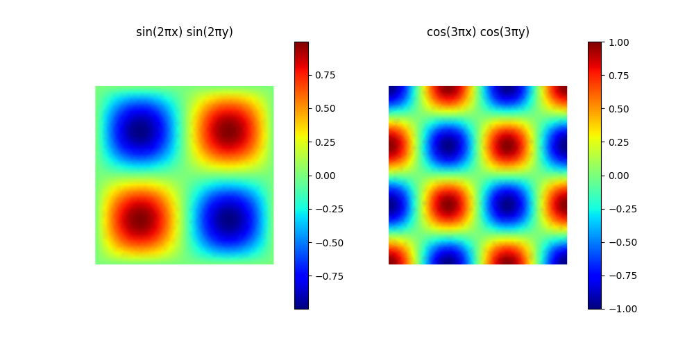
Fig. 4 mesh.plot({...}) with a multi-key dict renders one panel per field; each panel inherits a colourbar scaled to its own data range.

By default plot() only colour-fills the elements. Pass show_mesh=True to overlay the mesh wireframe (and, at order ≥ 2, the interpolation nodes) on top of the field — useful for sanity-checking a freshly solved problem:

mesh.plot({"u": u}, save_path="u.png", show_mesh=True)

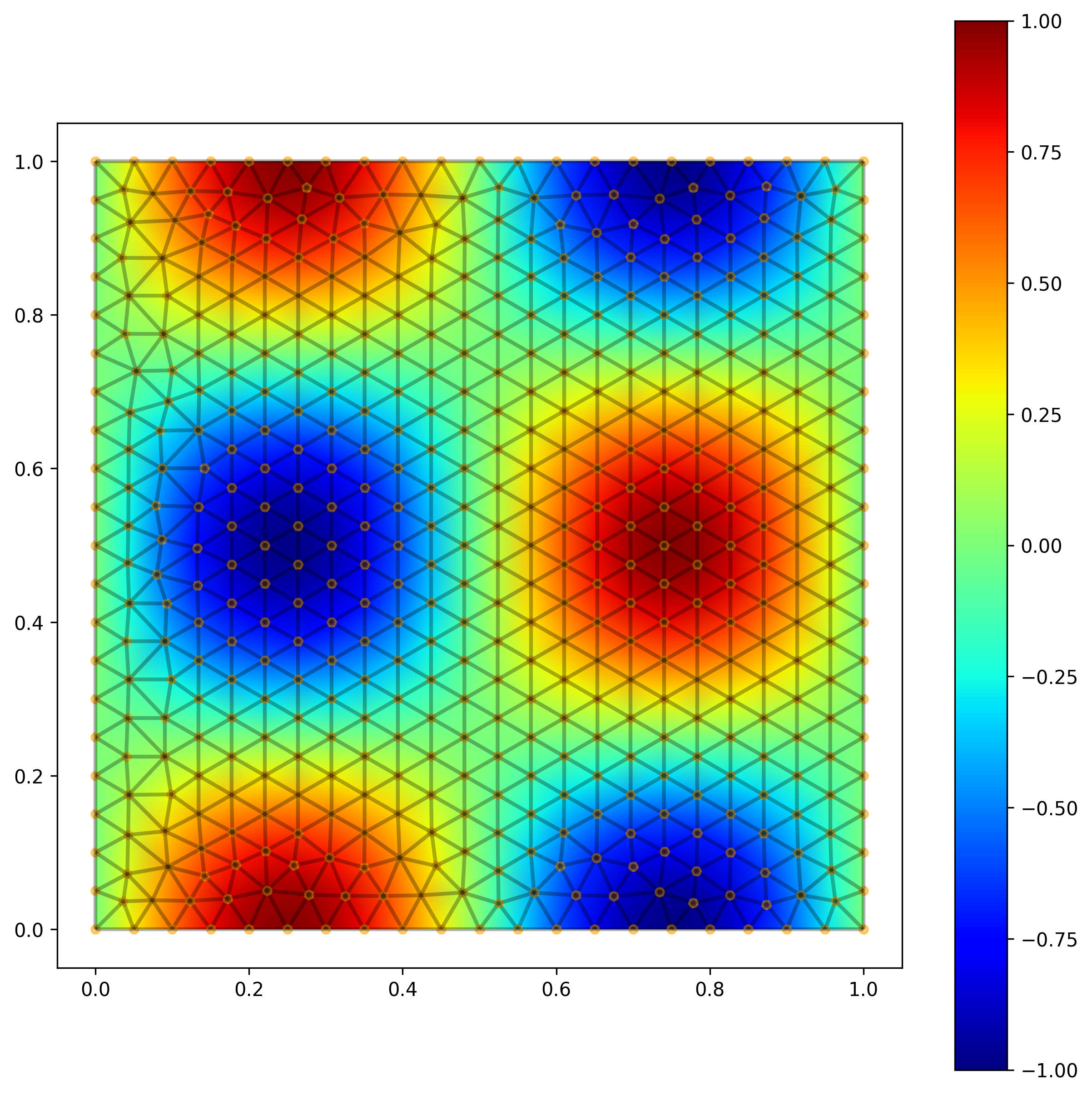
Fig. 5 mesh.plot({"u": u}, show_mesh=True) on a tri mesh. Without show_mesh=True the same call would show only the smooth colour fill, with no triangle edges or interpolation nodes drawn.

For a deep dive on visualization, including 3D deformation plots and animations, see the Example Gallery.

What’s next

• Elements and Quadrature — the reference shapes, basis evaluation, and the ordering convention behind reorder=True.

• Forms — turn a mesh into a stiffness matrix or load vector via the assembler base classes.

• Quickstart — a complete worked Poisson problem that uses everything on this page.