Complex-Valued FEM — Helmholtz

A single script, examples/wave/helmholtz/helmholtz.py, solves the time-harmonic (frequency-domain) Helmholtz equation on the unit square with a complex-valued coefficient. It is the end-to-end validation of the complex assembly path unblocked in ROADMAP item 2: a complex element matrix now flows all the way from a complex point_data coefficient, through assembly and Dirichlet condensation, into a complex linear solve — and back through a correct complex adjoint.

The strong form is the interior Helmholtz problem

\[-\Delta u(x, y) \;-\; k^2\, u(x, y) \;=\; 0 \quad \text{in } \Omega = (0,1)^2, \qquad u = g \text{ on } \partial\Omega,\]

driven entirely by the boundary data. We use the manufactured plane-wave solution

\[u_\text{exact}(x, y) \;=\; e^{\,i k x},\]

so the Dirichlet data is \(g = u_\text{exact}|_{\partial\Omega}\). The body force is exactly zero, because \(-\Delta e^{ikx} = k^2 e^{ikx}\) cancels the \(-k^2 u\) mass term pointwise — which makes the analytic solution available everywhere for an error check.

Why a complex example matters

Everything in the assembly stack used to assume a real dtype. Helmholtz is the smallest problem that exercises the complex path end to end:

• Complex coefficient through point_data. The wavenumber term \(k^2\) is carried as a (here constant, possibly complex) per-node field and broadcast over elements and quadrature inside ElementAssembler.__call__ — the same mechanism a PML layer will use for its anisotropic, spatially-varying complex coefficients.

• Complex Dirichlet condensation. The boundary values \(g\) are complex, so Condenser must carry a complex inner-system right-hand side.

• Complex linear solve. SparseMatrix.solve delegates to torch-sla’s complex-symmetric \(LDL^\top\) / Hermitian \(LDL^\mathsf{H}\) factorisations, which also supply the matching complex adjoint — essential for downstream gradient-based design.

TensorMesh setup

The weak form is a single bilinear assembler; the only thing that marks it as complex is the dtype cast and the complex k_sq coefficient:

Listing 10 examples/wave/helmholtz/helmholtz.py (essence)

class HelmholtzAssembler(ElementAssembler):
    # a(u, v) = ∫ ∇u·∇v - k² u v dΩ
    def forward(self, gradu, gradv, u, v, k_sq):
        return gradu @ gradv - k_sq * u * v

mesh = gen_rectangle(chara_length=h, element_type="tri")
points = mesh.points.to(torch.float64).to(device)

# k² as a complex per-node coefficient (constant here; a PML layer
# would make it anisotropic and spatially varying).
k_sq_field = torch.full((mesh.n_points,), k * k + 0j,
                        dtype=torch.complex128, device=device)

asm = HelmholtzAssembler.from_mesh(mesh, quadrature_order=3)
asm.type(torch.complex128).to(device)            # cast the assembler complex
H = asm(points=points, point_data={"k_sq": k_sq_field})

# Dirichlet g = u_exact on the boundary; the inner RHS is complex.
g = torch.exp(1j * k * mesh.points[:, 0].to(torch.float64)).to(torch.complex128)
condenser = Condenser(mesh.boundary_mask, dirichlet_value=g[mesh.boundary_mask])
H_inner, rhs_inner = condenser(H, torch.zeros(mesh.n_points, dtype=torch.complex128))
u = condenser.recover(H_inner.solve(rhs_inner))

Two points worth noting:

• The mesh stays real. Geometry, shape functions, and quadrature weights remain float64; only the coefficient and the resulting system are complex. asm.type(torch.complex128) promotes the assembler, and the real shape-function tensors are upcast to the coefficient’s complex dtype on demand inside the assembly einsum.

• ``complex128`` is the default. The convergence study runs in double-complex; --dtype complex64 is available but, as with real FEM, double precision is recommended for clean convergence rates.

Convergence

Refining the mesh drives the \(L^2\) error against \(u_\text{exact}\) down at the expected FEM rate (modulo the usual Helmholtz “pollution” at moderate \(k\)). At \(k = 2\pi\):

h=0.200  n_dofs=  44  L2 err = 1.529e-01
h=0.100  n_dofs= 143  L2 err = 5.274e-02
h=0.050  n_dofs= 509  L2 err = 1.506e-02
h=0.025  n_dofs=1934  L2 err = 3.935e-03

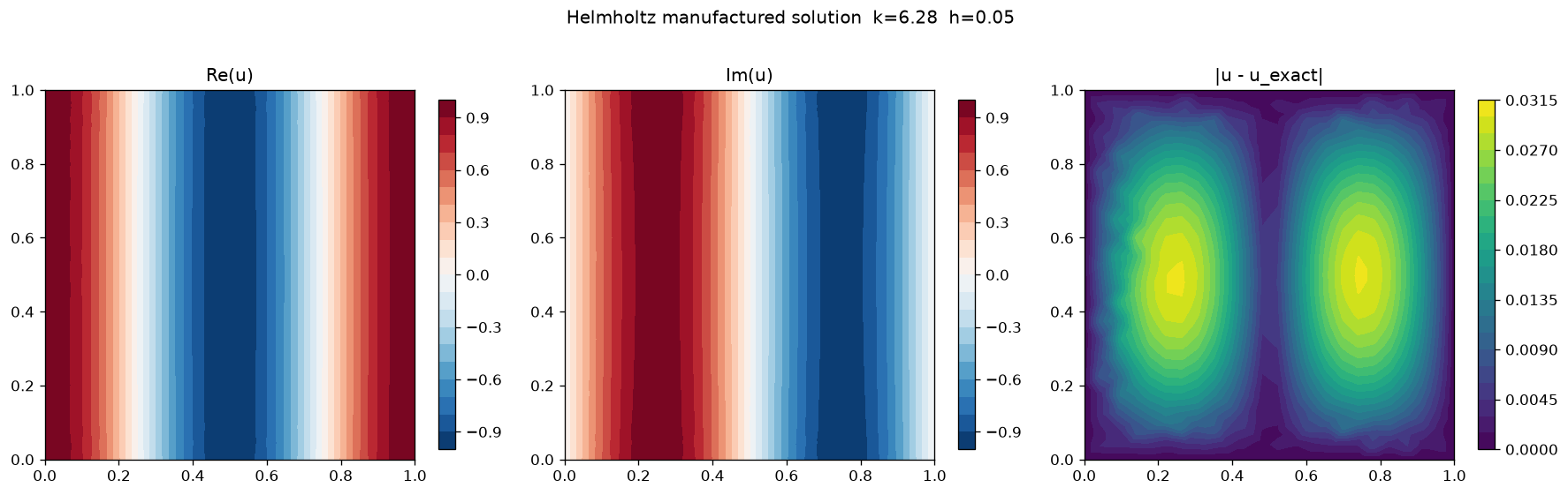
Fig. 42 helmholtz.py output at \(k = 2\pi\), \(h = 0.1\): the real part, imaginary part, and pointwise error \(|u - u_\text{exact}|\) of the computed field. The plane wave \(e^{ikx}\) propagates along \(x\); the error panel stays at the discretisation floor across the whole domain.

Cross-validation against scikit-fem

The strongest correctness signal for the complex path is an independent pipeline. tests/assemble/test_helmholtz_example.py hands the same (points, cells) to scikit-fem’s MeshTri, assembles the same form with its built-in laplace / mass integrators, solves with scipy.sparse.linalg.spsolve, and compares node by node. At \(h = 0.1\), \(k = 2\pi\) the two solvers agree to floating-point precision:

\[\frac{\max\,|u_\text{tensormesh} - u_\text{skfem}|}{\max\,|u|} \;\approx\; 2.3\times10^{-15},\]

i.e. machine \(\varepsilon\) — both pipelines inherit the same \(5.27\times10^{-2}\) discretisation error against the analytic plane wave.

Running the example

cd examples/wave/helmholtz
python helmholtz.py                                  # k = 2π, writes helmholtz.png
python helmholtz.py --k 12.566 --chara-length 0.05   # k = 4π
python helmholtz.py --no-plot                        # convergence table only

What’s next

• PML scattering. The constant scalar \(k^2\) here is the simplest complex coefficient. The same point_data channel already carries anisotropic complex tensor coefficients, so the natural next step is a perfectly-matched-layer absorbing boundary with coordinate-stretched \(A(x), c(x)\) and a scattering obstacle — see ROADMAP item 2.

• Metamaterial topology optimization. With the complex adjoint in place, the density → SIMP → filter pipeline from Inverse Design & Identification can be driven by a wave objective (e.g. \(|u|^2\) at a target point).

• Wave Equation — the time-domain counterpart: the real, hyperbolic wave equation with explicit central differences.