Cantilever Beam

The textbook entry-point for solid mechanics in TensorMesh: a
\(2.0 \times 0.2 \times 0.2\) m steel cantilever clamped at
one end, loaded by a downward force at the other. Linear
small-strain elasticity, one direct linear solve, ~30 lines of
code. The script is
examples/solid/cantilever_beam/cantilever_beam.py.
Problem
Small-strain linear elasticity:
where \(\mathbb{C}\) is the isotropic stiffness tensor with Young’s modulus \(E = 200\) GPa and Poisson’s ratio \(\nu = 0.3\). Boundary conditions:
clamp at \(x = 0\): \(\mathbf{u} = \mathbf{0}\),
tip load at \(x = 2\): total force \(F = -100\) kN distributed over the right face nodes,
all other surfaces: traction-free.
TensorMesh setup
The full driver:
from tensormesh import Mesh, Condenser
from tensormesh.dataset.mesh import gen_cube
from tensormesh.assemble import LinearElasticityElementAssembler
from tensormesh.material import Steel
from tensormesh.visualization import plot_deformation

# 1. Mesh
mesh = gen_cube(chara_length=0.08,
                left=0.0, right=2.0,
                bottom=0.0, top=0.2,
                front=0.0, back=0.2)

# 2. Material + stiffness assembly
K = LinearElasticityElementAssembler.from_mesh(
        mesh, E=Steel.E, nu=Steel.nu)()

# 3. Boundary conditions: clamp the x=0 face
eps = 1e-5
fixed_node_mask = torch.abs(mesh.points[:, 0]) < eps
fixed_dof_mask  = torch.repeat_interleave(fixed_node_mask, mesh.dim)
condenser       = Condenser(fixed_dof_mask)

# 4. Load: distribute -100 kN over the right-face nodes
right_mask  = torch.abs(mesh.points[:, 0] - 2.0) < eps
right_nodes = torch.where(right_mask)[0]
rhs = torch.zeros((mesh.n_points, mesh.dim))
rhs[right_nodes, 1] = -1e5 / right_nodes.shape[0]
rhs_flat = rhs.flatten()

# 5. Solve
K_, F_  = condenser(K, rhs_flat)
u_full  = condenser.recover(K_.solve(F_)).reshape(-1, mesh.dim)

# 6. Visualize the displaced mesh
plot_deformation(mesh, u_full,
                 save_path="cantilever_steel.png",
                 scale=50)
A few details that make this short:
LinearElasticityElementAssembleris a built-in vector-valued assembler — it returns a stiffness block of size[mesh.dim, mesh.dim]per (test, trial) basis pair, all wrapped into oneSparseMatrixof shape[mesh.dim * n_points, mesh.dim * n_points]. See Forms for the convention.The DOF layout is per-node
[u_x, u_y, u_z];torch.repeat_interleave(fixed_node_mask, dim)lifts the per-node mask to per-DOF.tensormesh.materialships predefined isotropic materials (Steel,Aluminum,Rubber,Bone) so you don’t have to memorize \(E\) and \(\nu\).plot_deformationexaggerates the deformation byscale=50for visibility — the actual tip displacement is on the order of millimeters.
Sanity check
For a tip-loaded prismatic cantilever, Euler-Bernoulli beam theory predicts a tip deflection
with \(L = 2\) m, \(b = h = 0.2\) m, \(E = 200\) GPa,
\(F = 10^5\) N. That gives \(\delta \approx 5.0\) mm.
The FEM solution at the right-face center should agree to within
the coarse-mesh approximation error (a few percent at
chara_length=0.08).
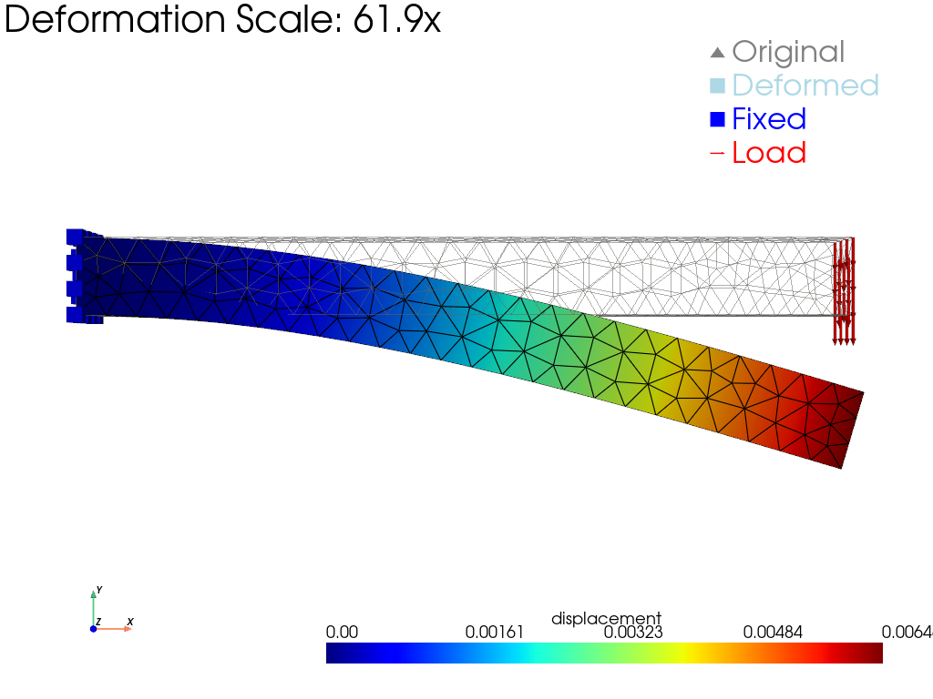
Fig. 59 Output of cantilever_beam.py. The undeformed beam is drawn
in light grey; the deformed configuration is colored by
displacement magnitude. Blue cubes mark fixed nodes at
\(x=0\); red arrows mark the distributed tip load on the
\(x=L\) face. The deformation is exaggerated by ~62× so the
bending is visible at this aspect ratio — the actual tip
displacement is on the order of millimeters and matches the
Euler-Bernoulli closed form to within the coarse-mesh
approximation error.
Running it
cd examples/solid/cantilever_beam
python cantilever_beam.py     # writes cantilever_steel.png
Console output reports the maximum nodal displacement in millimeters.
What’s next
Forms — vector-valued assembler return shapes (
[dim, dim]blocks per quadrature point).Boundary Conditions — DOF masking for vector unknowns.
Hyperelastic Beam (Neo-Hookean) — same geometry-style problem, but large deformation through a Neo-Hookean energy.