Magnetostatics (Maxwell)

A 3D magnetostatics problem: recover the magnetic field around a current-carrying wire by solving for the magnetic vector potential \(\mathbf{A}\) on the unit cube. The script examples/maxwell/magnetostatic.py uses continuous nodal Lagrange elements with the stabilized mixed formulation of Badia & Codina (2012) [BC2012], which makes the curl-curl problem well-posed on standard (non-curl-conforming) nodal spaces.

Note

TensorMesh ships continuous nodal Lagrange elements. The natural space for \(\nabla\times\nabla\times\) is the curl-conforming Nédélec edge element, which is not native yet — so this example takes the same pragmatic route as the lid-driven cavity: solve on equal-order nodal spaces and add consistent stabilization (here a Coulomb-gauge Lagrange multiplier plus grad-div and multiplier terms) to suppress the spurious modes. More specialized FE spaces will be added gradually.

Problem

Magnetostatics is Ampère’s law \(\nabla\times\mathbf{H}=\mathbf{J}\) together with \(\nabla\cdot\mathbf{B}=0\) and \(\mathbf{B}=\mu\mathbf{H}\). Writing \(\mathbf{B}=\nabla\times\mathbf{A}\) satisfies the divergence constraint identically and — with reluctivity \(\nu=1/\mu\) absorbed into a nondimensional scaling — reduces Ampère’s law to the curl-curl equation for \(\mathbf{A}\):

\[\nabla\times(\nabla\times\mathbf{A}) - \nabla p = \mathbf{J}, \qquad \nabla\cdot\mathbf{A} = 0 \quad\text{in } \Omega = (0,1)^3,\]

where the scalar \(p\) is a Lagrange multiplier enforcing the Coulomb gauge \(\nabla\cdot\mathbf{A}=0\). The gauge is not optional: the curl-curl operator annihilates every gradient field, so its kernel is enormous and \(\mathbf{A}\) is only unique up to \(\nabla\phi\) without it.

Boundary conditions are the homogeneous tangential trace

\[\mathbf{n}\times\mathbf{A}=\mathbf{0}, \qquad p = 0 \quad\text{on } \partial\Omega,\]

i.e. on each axis-aligned face the two tangential components of \(\mathbf{A}\) are fixed to zero (on \(x=0,1\) that is \(A_y\) and \(A_z\)), the constraints combining along the edges and corners.

Current source. A smooth \(z\)-directed channel through the centre of the cube — a soft model of a straight wire,

\[\mathbf{J} = J_0 \exp\!\left( -\frac{(x-x_c)^2+(y-y_c)^2}{2\sigma^2} \right)\,\mathbf{e}_z,\]

with \(J_0 = 100\), centre \((x_c, y_c) = (0.5, 0.5)\), and width \(\sigma = 0.08\). It is \(z\)-invariant, so \(\nabla\cdot\mathbf{J} = 0\); in free space such a current produces a purely azimuthal field circling the wire, which is the qualitative signature to look for.

Stabilized weak form

Find \((\mathbf{A}_h, p_h) \in V_h \times Q_h\) in continuous Lagrange spaces such that, for all \((\mathbf{v}_h, q_h)\),

\[\begin{split}a(\mathbf{A}_h,\mathbf{v}_h) + b(\mathbf{v}_h,p_h) + s_u(\mathbf{A}_h,\mathbf{v}_h) &= (\mathbf{J},\mathbf{v}_h), \\ -\,b(\mathbf{A}_h,q_h) + s_p(p_h,q_h) &= 0,\end{split}\]

with the forms

\[\begin{split}a(\mathbf{A},\mathbf{v}) &= (\nabla\times\mathbf{A},\,\nabla\times\mathbf{v})_\Omega, & b(\mathbf{v},p) &= -(\nabla p,\,\mathbf{v})_\Omega, \\ s_u(\mathbf{A},\mathbf{v}) &= \sum_{K\in\mathcal{T}_h} h_K^2\, (\nabla\cdot\mathbf{A},\,\nabla\cdot\mathbf{v})_K, & s_p(p,q) &= (\nabla p,\,\nabla q)_\Omega.\end{split}\]

The two stabilization terms are what make the nodal discretization robust: the grad-div penalty \(s_u\) controls the divergence of \(\mathbf{A}\), and \(s_p\) regularizes the multiplier — this is equation (3.6) of [BC2012]. The demo uses a constant length scale \(h^2 = \texttt{chara\_length}^2\) for every element. Assembled, the four forms become a 2×2 block saddle-point system

\[\begin{split}\begin{bmatrix} A + S_u & B \\ -B^\top & S_p \end{bmatrix} \begin{bmatrix} \mathbf{A}_h \\ p_h \end{bmatrix} = \begin{bmatrix} \mathbf{f} \\ \mathbf{0} \end{bmatrix}.\end{split}\]

TensorMesh setup

Each bilinear form is one small ElementAssembler whose forward returns the per-node block. The curl-curl form, for instance, builds the two skew-symmetric cross-product matrices \([\nabla N]_\times\) and contracts them — column \(a\) of \([\nabla N]_\times\) is exactly \(\nabla\times(N\,\mathbf{e}_a)\), so the contraction is the \([3,3]\) block \((\nabla\times\mathbf{u})\cdot(\nabla\times\mathbf{v})\):

Listing 20 examples/maxwell/magnetostatic.py (essence)

class CurlCurlAssembler(ElementAssembler):
    """(curl u, curl v) for 3D vector nodal fields."""
    def forward(self, gradu, gradv):
        zero = torch.zeros_like(gradu[0])
        curl_u = torch.stack((torch.stack((zero, -gradu[2], gradu[1])),
                              torch.stack((gradu[2], zero, -gradu[0])),
                              torch.stack((-gradu[1], gradu[0], zero))))
        curl_v = ...                       # the same, built from gradv
        return curl_u.T @ curl_v           # [3, 3] block

A  = CurlCurlAssembler.from_mesh(mesh)()
Su = DivergenceStabilizationAssembler.from_mesh(mesh, h2=h2)()   # h^2 (div u, div v)
Sp = PressureStabilizationAssembler.from_mesh(mesh)()            # (grad p, grad q)
B  = PressureCouplingAssembler.from_mesh(mesh)()                 # -(grad p, v)

K = SparseMatrix.combine([[A + Su, B],
                          [-1.0 * B.T, Sp]])

A few details worth flagging:

• Block assembly. SparseMatrix.combine tiles the four sparse blocks into the saddle-point matrix, so the vector \(\mathbf{A}\) DOFs and the scalar \(p\) DOFs share one linear system.

• Tangential BC as a DOF mask. tangential_vector_potential_mask builds the per-component Dirichlet mask for \(\mathbf{n}\times\mathbf{A}=\mathbf{0}\); concatenated with mesh.boundary_mask for \(p\), it feeds a single Condenser that condenses out every constrained DOF before the solve.

• Recovering the field. \(\mathbf{B}=\nabla\times\mathbf{A}\) is a derived, element-wise quantity. The script projects it back to a smooth nodal field by an \(L^2\) projection — assemble a MassElementAssembler, build the curl right-hand side with a NodeAssembler, and solve \(M\,\mathbf{B} = \tilde{\mathbf{B}}\) component-wise. This is the same recipe the cylinder flow uses to recover vorticity.

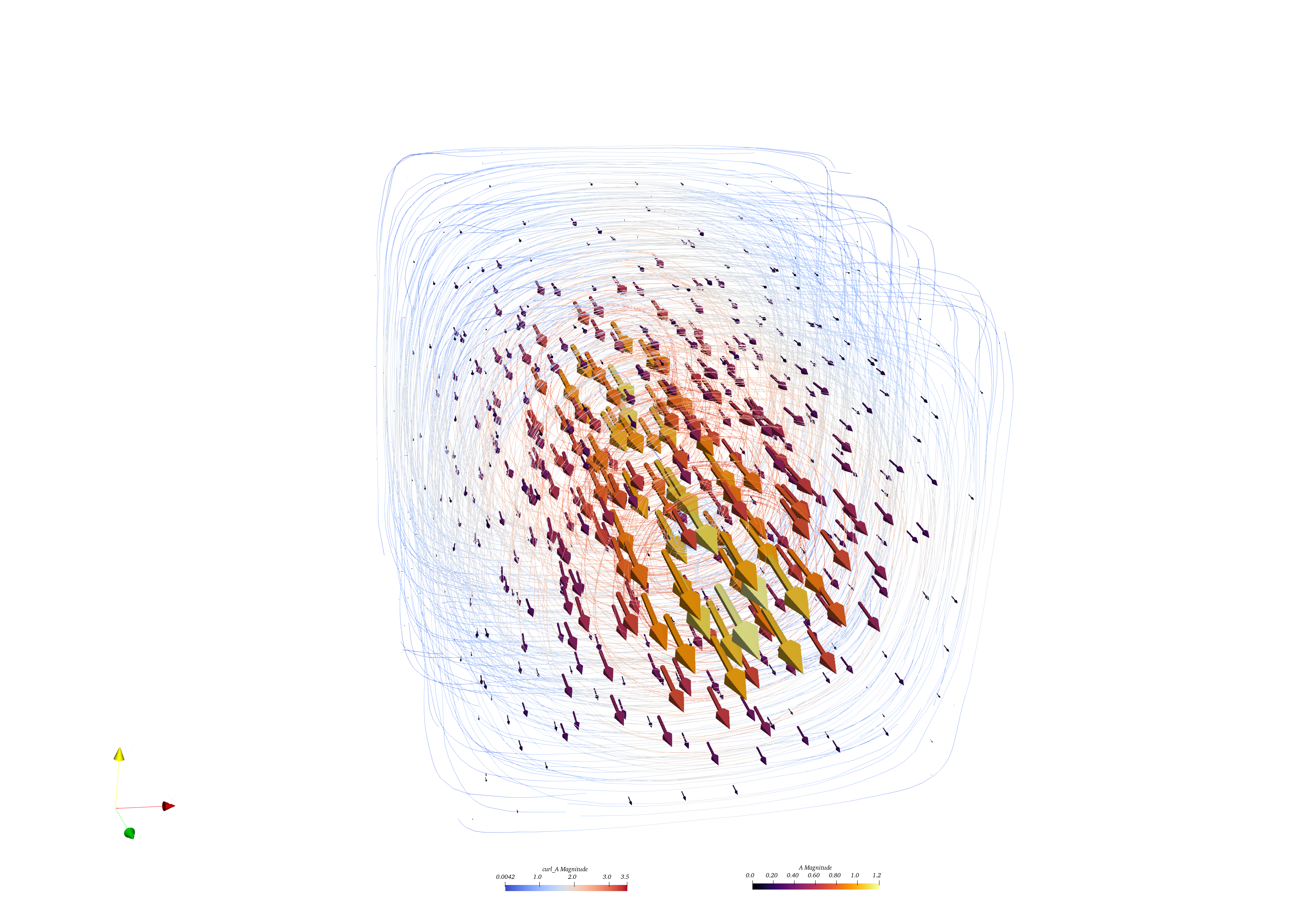
Fig. 50 Output of magnetostatic.py (rendered in ParaView): streamlines of \(\mathbf{B}=\nabla\times\mathbf{A}\), viewed roughly down the \(z\) axis. The warm glyphs at the centre mark the \(z\)-directed current channel; the field lines wrap azimuthally around it — the right-hand-rule pattern of a straight wire — while the finite cube boundary gently squares off the outer loops.

Running it

cd examples/maxwell
python magnetostatic.py        # writes magnetostatic_3d.vtu

The solve writes magnetostatic_3d.vtu with two nodal point fields, the vector potential A and the magnetic field curl_A \(= \nabla\times\mathbf{A}\). Open it in ParaView and apply Stream Tracer or Glyph to curl_A to reproduce the figure above. The mesh size and current settings live at the top of main() if you want to experiment.

What’s next

• Lid-Driven Cavity — the same “equal-order nodal + consistent stabilization” strategy, there to satisfy the incompressible Navier-Stokes inf-sup condition.

• Forms — vector-valued forward returns and the per-node block convention shared by every assembler here.

• Boundary Conditions — DOF masking and static condensation for vector unknowns.

[BC2012] (1,2)

S. Badia and R. Codina, A Nodal-based Finite Element Approximation of the Maxwell Problem Suitable for Singular Solutions, SIAM Journal on Numerical Analysis, 50(2):398–417, 2012.