Forms

Solving a PDE in TensorMesh starts with two pieces of math:

\[a(u, v) \;=\; \int_{\Omega} \cdots \, \mathrm{d}\Omega \qquad l(v) \;=\; \int_{\Omega} \cdots \, \mathrm{d}\Omega\]

The bilinear form \(a(u, v)\) becomes a stiffness matrix; the linear form \(l(v)\) becomes a load vector. In TensorMesh you write each integrand as a single Python function and the library handles quadrature, geometry, and the global scatter into a sparse matrix or vector. This is the layer most users interact with — once you have worked through this page you can express almost any FEM weak form in a few lines of Python.

Three base classes cover the common cases. The choice depends on the shape of the object you want to assemble:

Base class	Math object	Output	Typical use
ElementAssembler	bilinear form \(a(u, v)\)	SparseMatrix	stiffness, mass, elasticity, advection-diffusion, …
NodeAssembler	linear form \(l(v)\)	1-D torch.Tensor	body forces, RHS of \(L^2\) projections, residuals, …
FacetAssembler	surface integral	1-D torch.Tensor	Neumann tractions, penalty contact, Robin BCs, surface tension, …

All three share the same dispatch contract for forward(...), the same from_mesh(...) / from_assembler(...) constructors, and the same call-time data plumbing. Learn the contract once and the three classes feel like a single tool.

The weak-form contract

Every assembler subclass overrides forward(...). The base class inspects the parameter names of your function and supplies the right tensor for each one, evaluated at every quadrature point of every element. The bookkeeping — Jacobians, basis values, quadrature weights, global scatter — happens behind the scenes.

Argument name	Provided by	Per-point shape	Notes
u, v	the basis itself at one quadrature point	0D [] (Element / Node) or 1D [B] (Facet)	the inner vmap layer turns this into a scalar in Element / Node forward
gradu, gradv	basis gradient in physical coordinates	1D [D] (Element / Node) or 2D [B, D] (Facet)	already the physical-space gradient — the \(J^{-T}\) chain rule is applied for you
x	physical coordinate at the quadrature point	1D [D]	auto-supplied from mesh.points; no need to pass it explicitly
any key in point_data	your nodal tensor interpolated to the quadrature point	[...] (per-node trailing dims preserved)	e.g. pass point_data={"kappa": kappa} then use kappa as a forward parameter
grad + key in point_data	gradient of that field at the quadrature point	[..., D]	automatic — request it by name, do not pass anything extra
any key in element_data	per-element constant or per-(element, quadrature) varying tensor	[...]	good for history variables in plasticity or pre-computed cell parameters
any key in scalar_data	global scalar	scalar	passed verbatim (no vmap broadcasting); use for time steps, penalty weights, …

Inside forward you write the integrand as a normal tensor expression. The base class:

1. broadcasts your function across elements and quadrature points (using torch.vmap()),

2. multiplies the returned integrand by \(|\det J|\,w\) (the JxW per quadrature point — see Elements and Quadrature),

3. scatters the result into the right global slot.

The dispatch is by name, not by position — forward(self, u, v) and forward(self, v, u) are equivalent. The contract only fails if you use an unrecognised name; you will get a clear ValueError at call time pointing to the bad argument.

Tip

You never call forward yourself. The library calls it under vmap for every quadrature point of every element, so even a trivial print(u) inside forward will fire \(N_e \times N_q\) times and produce strange-looking traced tensors. For debugging weak forms, set batch_size=1 and call the assembler on a one-element mesh, or check the assembled output directly with K.to_dense().

ElementAssembler — bilinear forms

For a(u, v), write a forward(...) that returns the integrand and call from_mesh(...) + (). Calling the assembler returns a SparseMatrix.

from tensormesh import Mesh, ElementAssembler

class LaplaceAssembler(ElementAssembler):
    r"""a(u, v) = ∫ ∇u · ∇v dΩ"""
    def forward(self, gradu, gradv):
        return gradu @ gradv

mesh = Mesh.gen_rectangle(chara_length=0.15)
K = LaplaceAssembler.from_mesh(mesh)()
K.shape
# (143, 143)

That’s the whole user story for a scalar bilinear form: one forward method, three lines of glue, sparse matrix in hand.

The full call signature is

__call__(points=None, func=None, point_data=None,
         element_data=None, scalar_data=None, batch_size=-1)

with all arguments optional. The mesh’s own points are used when points=None; func lets you swap in a different integrand without defining a new subclass (handy in inverse problems where the bilinear form is a moving target); the three *_data dicts plumb call-time inputs into your forward parameters (see Choosing where call-time parameters live); batch_size is a memory knob covered in Memory batching with batch_size.

Parameters that vary by mesh: point_data, element_data, scalar_data

Most weak forms involve coefficients beyond just \(u, v, \nabla u, \nabla v\). The three call-time dicts let you pass them in without changing the assembler class itself:

import torch

kappa_field = torch.rand(mesh.n_points, dtype=mesh.dtype)  # spatially varying coef

class WeightedLaplace(ElementAssembler):
    def forward(self, gradu, gradv, kappa):
        # `kappa` has shape [] at each quadrature point — interpolated
        # from the nodal values via the same basis functions used for u, v.
        return kappa * (gradu @ gradv)

K = WeightedLaplace.from_mesh(mesh)(point_data={"kappa": kappa_field})

You can also bake parameters into the subclass via __post_init__, which runs once after the projector + quadrature are wired up:

class ScaledLaplace(ElementAssembler):
    def __post_init__(self, alpha=1.0):
        self.alpha = alpha

    def forward(self, gradu, gradv):
        return self.alpha * (gradu @ gradv)

K = ScaledLaplace.from_mesh(mesh, alpha=2.5)()         # alpha is a constructor kw

Either pattern works; pick whichever matches the lifetime of the parameter (constant across many solves → __post_init__; varies from call to call → call-time dict).

Sparsity: what the assembled output actually looks like

The SparseMatrix is COO-format on top of torch_sla.SparseTensor; you can @ against it, .solve(b) against it, or densify it for inspection. The two panels below show the sparsity pattern of the Laplace stiffness above, next to the 2D-elasticity stiffness on the same mesh:

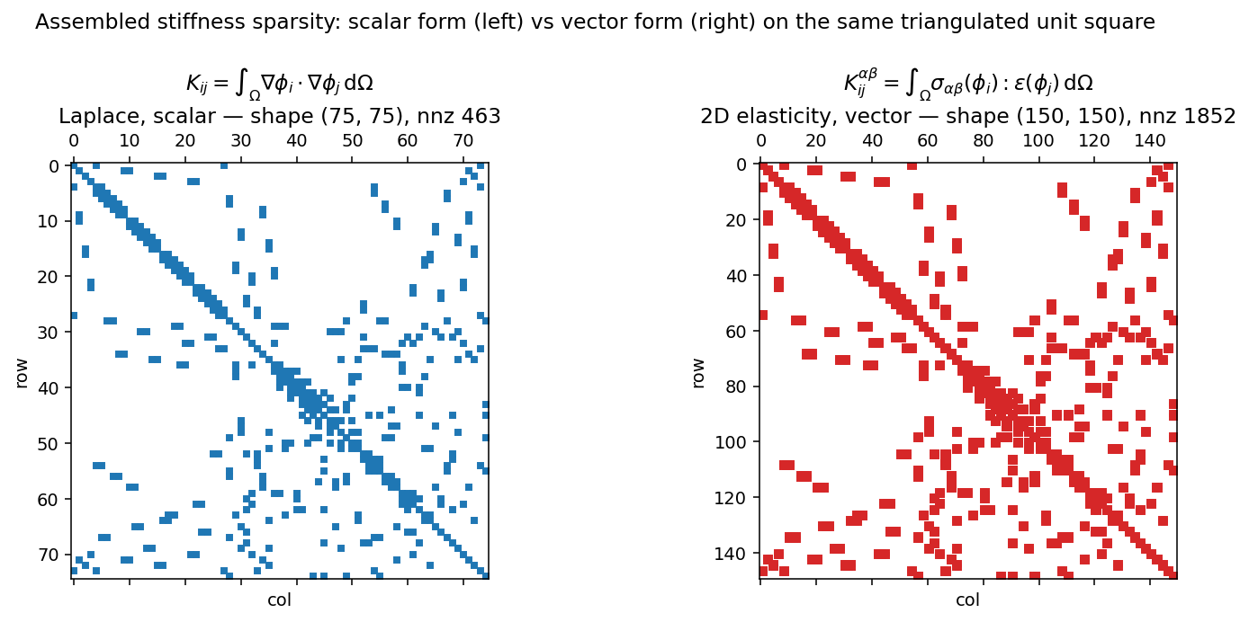
Fig. 8 The scalar Laplace stiffness has one entry per (i, j) adjacent node pair. The 2D-elasticity stiffness has the same connectivity but each entry is now a \(2 \times 2\) block (one row/col per displacement component), giving a matrix four times larger with sixteen times the non-zeros. The library detects the block structure from the rank of your forward return — see the next section.

Vector-valued forms and block-CSR output

For vector-valued problems (linear elasticity, Stokes velocity blocks, electromagnetics in vector form) each node carries \(H > 1\) degrees of freedom. The bilinear form integrand for an entry \((i, j)\) is then a \(H \times H\) block, and the assembled matrix has shape \([N_\text{points}\, H,\, N_\text{points}\, H]\).

The library decides scalar vs block by inspecting the rank of what your forward returns:

• forward returns a 2-D tensor [B, B] → scalar, output shape \([N_\text{points}, N_\text{points}]\);

• forward returns a 4-D tensor [B, B, H, H] → block, output shape \([N_\text{points}\, H, N_\text{points}\, H]\).

For linear elasticity in 2D, the integrand at a quadrature point is

\[K_{ij}^{\alpha\beta} \;=\; \int_\Omega \mathbf{B}_i^T\, \mathbf{C}\, \mathbf{B}_j \,\mathrm{d}\Omega, \qquad \mathbf{B}_i \;=\; \text{Voigt}(\nabla \phi_i),\]

which is exactly the built-in LinearElasticityElementAssembler:

import tensormesh.functional as F

class Elasticity(ElementAssembler):
    def __post_init__(self, E=1.0, nu=0.3):
        self.E, self.nu = E, nu
    def forward(self, gradu, gradv):
        Ba = F.voigt_shape_grad(gradu)              # [3, dim*dim] in 2D
        Bb = F.voigt_shape_grad(gradv)
        C  = F.voigt_stiffness(self.E, self.nu, dim=gradu.shape[0])
        C  = C.to(dtype=gradu.dtype, device=gradu.device)
        return Ba.T @ C @ Bb                        # [dim, dim] block

The whole 2D mesh of 143 nodes produces a \(286 \times 286\) stiffness — see the right panel of the figure above. Everything you read about scalar problems on this page applies unchanged to block problems; only the matrix shape grows.

NodeAssembler — linear forms

For \(l(v)\), the same pattern but with a single basis and a vector result:

import math, torch
from tensormesh import NodeAssembler

class L2Source(NodeAssembler):
    r"""b_i = ∫ f(x) φ_i dΩ for f(x, y) = sin(π x) sin(π y)."""
    def forward(self, x, v):
        return torch.sin(math.pi * x[0]) * torch.sin(math.pi * x[1]) * v

mesh = Mesh.gen_rectangle(chara_length=0.05)
b = L2Source.from_mesh(mesh)()                     # torch.Tensor [n_points]

Call signature:

__call__(points=None, func=None, point_data=None,
         scalar_data=None, batch_size=1)

Note that element_data is not accepted (linear forms rarely need per-element scratch data), and that the default batch_size is 1 rather than the -1 used by ElementAssembler. To disable batching here pass batch_size=-1 or batch_size=None; see Memory batching with batch_size for details.

End-to-end check: combining mass + load to project a function into the FE space. The mass matrix \(M\) is SPD, so we can invert it without Dirichlet conditions:

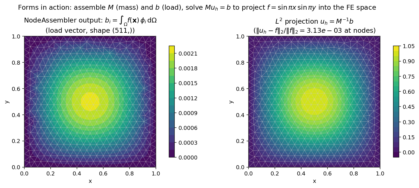
Fig. 9 Left: the assembled load vector \(b_i = \int_\Omega f\, \phi_i\, \mathrm{d}\Omega\), plotted as colored nodal values on the mesh. Right: the \(L^2\) projection \(u_h = M^{-1} b\). The nodal-error magnitude of ~3 × 10^-3 matches the expected \(O(h^2)\) discretisation error for P1 elements on this mesh.

This is the smallest possible “weak form → assembled output → solved field” loop; the more general workflow with boundary conditions and linear-solver options is the topic of Boundary Conditions and Sparse Solvers.

The simplest possible load — a constant body force \(\int c\, v\, \mathrm{d}\Omega\) — ships pre-built as const_node_assembler(); see Built-in assemblers.

FacetAssembler — boundary integrals

For surface terms — Neumann tractions, Robin BCs, penalty contact — FacetAssembler runs the same dispatch over facet quadrature instead of volume quadrature. The signature contract is identical to NodeAssembler’s except that the basis arguments u, v, gradu, gradv keep their basis dimension explicitly (1D [B] or 2D [B, D]):

from tensormesh import FacetAssembler

class IntegrateOne(FacetAssembler):
    r"""b_i = ∫_∂Ω φ_i dS — the per-node boundary-integral weights."""
    def forward(self, v):
        return v

mesh = Mesh.gen_rectangle(chara_length=0.1)
b = IntegrateOne.from_mesh(mesh)()
b.sum().item()                                     # 4.0 (exact perimeter of [0,1]^2)

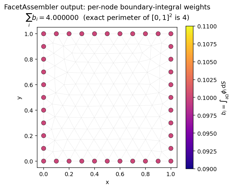
Fig. 10 The assembled vector b has support only on the boundary nodes (interior entries are zero). Summing all entries recovers the perimeter exactly. FacetAssembler defaults to integrating over mesh.boundary_mask; pass boundary_mask=... to from_mesh to restrict to a labelled sub-boundary.

Call signature:

__call__(points=None, func=None, point_data=None)

(no element_data, scalar_data, or batch_size for facet forms.) A worked penalty-contact example using ContactAssembler (a facet energy assembler) lives in the Example Gallery.

Choosing where call-time parameters live

Three dicts — point_data, element_data, scalar_data — cover every flavour of “data that varies across the mesh and is not part of the basis itself”. The decision tree:

You have a value …	Pass it as	It enters forward as	Examples
per node, with one trailing field shape	point_data={"kappa": kappa}	kappa (shape [...], interpolated to the quadrature point) and gradkappa (shape [..., D])	material coefficient defined at nodes, displacement field from a previous solve
per element (one value per cell)	element_data={"E": E} or element_data={"E": {"triangle": E_tri}}	the whole per-element slice (shape [...]); same value at every quadrature point inside that cell	per-cell Young’s modulus, marker labels, any quantity constant on the element
per (element, quadrature point) — .energy() path only	element_data={"eps_p": eps_p} with shape [n_elem, n_quad, ...]	the value at the current quadrature point (shape [...])	plastic strain history in J2Plasticity
global scalar	scalar_data={"dt": dt}	the scalar value (no vmap broadcasting)	time step \(\Delta t\), penalty weight \(\kappa\)

The name of the dict key becomes the parameter name in forward; the same name must not collide with a built-in (u, v, gradu, gradv, x, gradx). For point_data keys, you can also request the gradient by prefixing "grad" to the name — no extra plumbing is needed.

Caution

Per-(element, quadrature) element_data is auto-detected only by ElementAssembler.energy (see Energy-based assemblers (element_energy + .energy())), not by the matrix-assembling ElementAssembler.__call__ path. If you pass a tensor of shape [n_elem, n_quad, ...] to __call__, the whole [n_quad, ...] slice is handed to forward for each element — not the per-quadrature value. For matrix assembly today, keep element_data strictly per-element.

Feature matrix

The four call paths do not all support every plumbing knob. Use this table when you’re unsure whether a feature is available on the assembler you have:

Feature	Element __call__	Element .energy()	Node __call__	Facet __call__	Notes
points override	✓	✓	✓	✓	all paths re-cache the Transformation on new points
func override	✓	✓	✓ (forces vmap path)	✓	Node with compile() falls back to vmap when func is set
point_data keys + grad + key	✓	✓	✓	✓	same nodal-interpolation contract everywhere
per-element element_data	✓	✓	✗	✗	Node / Facet __call__ signatures don’t take it
per-(element, quadrature) element_data	✗ (whole slice)	✓ (auto-detect by shape[1] == n_quad)	✗	✗	only .energy() recognises the per-quadrature layout
scalar_data	✓	✓	✓	✗	facet integrals don’t take it
batch_size	✓ (default -1)	✓ (default -1)	✓ (default 1, disable with -1 or None)	✗	see Memory batching with batch_size for the per-class disable sentinels
.compile() fast path	✗	✗	✓ (single element type, no func)	✗	falls back to vmap when conditions aren’t met

Built-in assemblers

The most common forms are pre-written so you don’t have to. All of them are importable directly from tensormesh:

Class / factory	Kind	What it computes
LaplaceElementAssembler	Element	\(\int \nabla u \cdot \nabla v\, \mathrm{d}\Omega\) — Laplacian / diffusion stiffness
MassElementAssembler	Element	\(\int u\, v\, \mathrm{d}\Omega\) — mass matrix (transient, \(L^2\) projection)
LinearElasticityElementAssembler	Element (vector)	small-strain isotropic elasticity (parameters E, nu)
NeoHookeanModel	Element (energy)	Neo-Hookean hyperelasticity strain energy density
J2Plasticity	Element (energy)	\(J_2\) plasticity with isotropic hardening, return-mapping
ContactAssembler	Facet (energy)	base class for penalty / barrier contact and surface terms
const_node_assembler()	Node (factory)	\(\int c\, v\, \mathrm{d}\Omega\) — uniform body force; returns a class
func_node_assembler()	Node (factory)	\(\int f(\mathbf{x})\, v\, \mathrm{d}\Omega\) — spatially varying load; returns a class

Factory style for the node loads:

from tensormesh import const_node_assembler, func_node_assembler

ConstantLoad = const_node_assembler(c=9.81)
b = ConstantLoad.from_mesh(mesh)()

SineSource = func_node_assembler(lambda x: torch.sin(math.pi * x[..., 0]))
b = SineSource.from_mesh(mesh)()

The factories exist because Python class objects can’t be partially applied; a factory returns a freshly minted subclass that bakes the constant or function into __post_init__.

Energy-based assemblers (element_energy + .energy())

For nonlinear materials the most natural quantity to define is the strain energy density \(\Psi\), not the residual or stiffness:

\[\Pi(\mathbf{u}) \;=\; \int_\Omega \Psi(\nabla \mathbf{u})\, \mathrm{d}\Omega, \qquad \mathbf{f}_\text{int} \;=\; \frac{\partial \Pi}{\partial \mathbf{u}}, \qquad \mathbf{K}_\text{tan} \;=\; \frac{\partial^2 \Pi}{\partial \mathbf{u}^2}.\]

ElementAssembler supports this pattern via a parallel method, ElementAssembler.energy, that integrates an element_energy override and returns a scalar torch.Tensor. Because the entire pipeline is differentiable, E.backward() populates u.grad with the internal force vector, and torch.autograd.functional.hessian() (or a Krylov-friendly Hessian-vector product) gives the tangent stiffness:

from tensormesh.assemble import NeoHookeanModel

mesh = Mesh.gen_cube(chara_length=0.2)
model = NeoHookeanModel.from_mesh(mesh, E=1e6, nu=0.45)

u = torch.zeros_like(mesh.points, requires_grad=True)
E = model.energy(point_data={"displacement": u})
E.backward()
F_internal = u.grad                                # internal force vector

Use the matrix-based path (__call__ returning a SparseMatrix) for linear and bilinear-symmetric problems where you already have a closed-form integrand; use the energy path for hyperelasticity, plasticity, and any case where autograd through the constitutive law is the cleanest expression of the physics.

A custom form: reaction-diffusion

Combining stiffness and mass in one assembler:

\[a(u, v) \;=\; \int_{\Omega} \nabla u \cdot \nabla v \;+\; \kappa \, u v \, \mathrm{d}\Omega\]

is just two terms inside forward:

class ReactionDiffusion(ElementAssembler):
    def __post_init__(self, kappa=1.0):
        self.kappa = kappa

    def forward(self, u, v, gradu, gradv):
        return gradu @ gradv + self.kappa * (u * v)

K = ReactionDiffusion.from_mesh(mesh, kappa=2.5)()

Argument order doesn’t matter — the dispatch is by name. Mixing in point_data is just more parameters:

class WeightedReactionDiffusion(ElementAssembler):
    def forward(self, gradu, gradv, u, v, kappa, reaction):
        return kappa * (gradu @ gradv) + reaction * (u * v)

K = WeightedReactionDiffusion.from_mesh(mesh)(
    point_data={"kappa": kappa_field, "reaction": r_field}
)

This generalises straightforwardly: anything you can write as one algebraic expression in PyTorch can go inside forward, as long as the return shape obeys the contract in The weak-form contract.

Memory batching with batch_size

For very fine meshes or high-order elements, holding all per-element quadrature tensors in memory at once may not fit. The assembler __call__ accepts a batch_size argument that splits the quadrature dimension into chunks and accumulates the contribution:

K = LaplaceAssembler.from_mesh(mesh)(batch_size=4)

This is a memory knob, not problem-level vectorisation; for the latter see Batched Workflows.

How to disable batching:

• ElementAssembler — default batch_size=-1 processes all quadrature at once.

• NodeAssembler — default batch_size=1 processes one quadrature point at a time; pass -1 or None to disable batching and process all quadrature points at once.

• FacetAssembler — does not expose batch_size; facet integrals are small enough that batching has not been needed.

Any positive integer batch_size produces the same assembled result as the un-batched call. When batch_size does not evenly divide the per-element quadrature count, the loop runs one extra (shorter) batch on the tail; values larger than n_quadrature simply collapse to a single full batch.

Speeding up NodeAssembler with compile

NodeAssembler ships a fast path that bypasses torch.vmap() and uses direct broadcast operations instead. Enable it by chaining compile():

class Ones(NodeAssembler):
    def forward(self, v):
        return v

# Default — uses vmap dispatch (predictable, slowest startup):
asm = Ones.from_mesh(mesh)
b = asm()

# Compile mode — bypass vmap, use direct broadcast (5–30× faster in tight loops):
asm = Ones.from_mesh(mesh).compile()
b = asm()

# Disable for debugging (so breakpoints inside `forward` fire as expected):
asm.reset_compile()

The mode argument additionally controls whether torch.compile is layered on top: "disable" (default) does the vmap bypass only, "default" / "reduce-overhead" / "max-autotune" enable torch.compile with the given level of optimisation. For most users the default compile() (no torch.compile) is already a large speedup with no warm-up cost. flat_mode() is a synonym for compile(mode="disable").

The fast path only fires when all three of the following hold; if any of them fails the call falls back transparently to the vmap path:

1. .compile() has been called on the assembler (is_compiled returns True).

2. The mesh has exactly one element type (len(self.element_types) == 1). Mixed-element meshes use the vmap path even with compile enabled.

3. No func= override is passed at call time. Calling asm(func=alt_form) always goes through the vmap path so that you can swap integrands without recompiling.

Note

The fast path replaces vmap with explicit broadcast operations, which imposes a stricter contract on forward: it must work when v / gradv arrive with leading [n_quadrature, ...] / [n_element, n_quadrature, ...] dimensions rather than as scalars. Closed-form forms that compose those tensors via element-wise ops (return v, return gradv @ vec) work as-is; forms that index or reshape per-quadrature inputs may need a few broadcast tweaks, or are simpler to leave on the default vmap path. The fast path also does not auto-supply x; if you need coordinates, pass them in under a custom name (point_data={"xy": mesh.points} then forward(self, xy, v)).

Writing your own assembler

The library’s design assumes most users will, at some point, write a custom assembler. Here is the practical recipe.

1. Pick the base class by what you’re assembling — a matrix (ElementAssembler), a load vector (NodeAssembler), or a boundary term (FacetAssembler). If the integrand is most naturally expressed as a scalar energy density, use the .energy() path on ElementAssembler instead of writing the residual + stiffness by hand — autograd will do that for you.

2. Implement ``forward(self, …)``. Use only the parameter names listed in The weak-form contract (u, v, gradu, gradv, x, gradx), plus any keys you intend to pass through point_data, element_data, scalar_data. Return the per-point integrand at the right rank: scalar problems return [B, B] (Element) or [B] (Node / Facet); block problems return [B, B, H, H] or [B, H].

3. Stash parameters in ``__post_init__``, not __init__. The base class’s __init__ wires up the projector, transformation, and edges; __post_init__ runs immediately after with the constructor kwargs and is where self.E = E belongs.

4. Build the assembler via from_mesh() and call it. Constructor kwargs are forwarded to __post_init__. The instance is callable (and is an torch.nn.Module, so .to(device) / .double() Just Work).

A self-contained template covering both styles:

from tensormesh import Mesh, ElementAssembler

class MyForm(ElementAssembler):
    r"""a(u, v) = ∫ α ∇u · ∇v + β u v dΩ.

    α is a per-element coefficient, β a global scalar.
    """
    def __post_init__(self, beta=1.0):
        self.beta = beta

    def forward(self, gradu, gradv, u, v, alpha):
        return alpha * (gradu @ gradv) + self.beta * (u * v)

mesh   = Mesh.gen_rectangle(chara_length=0.1)
alpha  = torch.rand(mesh.cells["triangle"].shape[0], dtype=mesh.dtype)  # per-cell coef

K = MyForm.from_mesh(mesh, beta=2.5)(
    element_data={"alpha": alpha},
)

Debugging tips

• If the dispatch fails with ValueError: <name> is not supported, the parameter name doesn’t match any built-in or any key you passed in the data dicts. Check for typos like grad_u vs gradu or displacment vs displacement.

• If you hit a shape error inside forward, set batch_size=1 and call the assembler on a one-element mesh; the tensors handed in are then small enough to print and reason about. Remember that forward runs under vmap — what you see has the leading element / quadrature dimensions stripped.

• For sanity-checking the assembled output, run a known integral: a MassElementAssembler should give 1^T M 1 == area for the unit function; a FacetAssembler returning v should sum to the boundary length; a LaplaceElementAssembler applied to a linear field u = x should yield zero residual. The tests/assemble/test_facet.py file has a battery of these closed-form checks.

For exhaustive examples covering hyperelasticity, plasticity, contact, and fluid problems, see the Example Gallery.

What’s next

• Boundary Conditions — apply Dirichlet BCs to the matrix and vector you just assembled.

• Sparse Solvers — solve K x = b with the right backend.

• Differentiability — backprop a loss through assembly and solve, for inverse problems and topology optimisation.

• Batched Workflows — go from “one mesh per call” to “thousands of meshes per call” for ML dataset generation.

• Example Gallery — worked examples for elasticity, hyperelasticity, plasticity, contact, and fluids.