Hertzian Contact
A 2D contact-mechanics problem: a circular elastic indenter is
pressed into a rectangular elastic block; the contact pressure
along the interface should match the analytical Hertz solution.
The script examples/solid/hertzian_contact/hertzian_contact.py
solves it with a penalty method — the contact constraint is
enforced by adding a quadratic penalty energy to the total
potential, then minimized with L-BFGS.
Problem
Two linear-elastic bodies (\(E = 1000\) Pa, \(\nu = 0.3\)):
Indenter — full circular disc of radius \(R = 1.0\), meshed with Tri6 quadratic triangles, centered at \((-1.0, 0)\) so the right-most point sits at the origin. Its left-most arc (\(x < -1.8\)) is clamped.
Block — rectangle \([0, 1] \times [-1, 1]\), meshed with Quad9 quadratic quadrilaterals. The right edge (\(x = 1\)) has prescribed displacement \(u_x = -0.15\) (pushing left, into the indenter).
The contact interface is the vertical line \(x = 0\). As the block moves leftward the indenter is compressed, and a contact patch forms.
Penalty contact
Frictionless normal contact is the constraint \(g(\mathbf{x}) \geq 0\), where \(g\) is the gap function (signed distance between the two surfaces, positive when separated). The penalty method replaces the inequality constraint by the contact energy
where \(\langle x \rangle_+ = \max(x, 0)\) and \(k_p = 2 \times 10^6\) is the penalty stiffness. As \(k_p \to \infty\) the constraint is enforced exactly, but the problem becomes ill-conditioned; in practice \(k_p\) is chosen to be a few orders of magnitude larger than the elastic stiffness.
The total energy minimized at each L-BFGS step is
The first two terms come from
LinearElasticityElementAssembler ‘s
energy form (small-strain quadratic energy); the contact term is
implemented separately in the script.
Point-to-segment detection
The interface \(\Gamma_c\) is partitioned into “slave nodes” on one body and “master segments” on the other. For each slave node, the script projects onto the closest master segment, computes the signed normal gap, and accumulates the penalty contribution.
The script does this two-way (each body’s interface nodes are slaves with respect to the other body) which gives a symmetric formulation and avoids the bias of a one-master-one-slave choice.
Energy minimization with L-BFGS
The pattern is the one introduced in Hyperelastic Beam (Neo-Hookean): a
single u parameter for both meshes, BCs enforced inside the
closure, autograd providing the gradient. The contact term is
re-evaluated every iteration because the gap function depends on
the current configuration:
def closure():
    optimizer.zero_grad()
    u_active = apply_bcs(u)
    E_elastic_1 = model_circle.energy(...)
    E_elastic_2 = model_block.energy(...)
    E_contact   = penalty_contact_energy(u_active, k_p)
    total = E_elastic_1 + E_elastic_2 + E_contact
    total.backward()
    return total

for it in range(25):
    optimizer.step(closure)
Comparison with the Hertz analytical solution
For 2D plane-strain contact between an elastic cylinder and a half-space, Hertz theory gives a parabolic pressure distribution:
with effective modulus \(E^*\) and effective radius
\(R^*\) derived from the two-body geometry. The script extracts
the contact pressure from the converged solution and overlays it
on the analytical curve in hertzian_contact.png — the FEM
match is good once the mesh is fine enough near the contact patch
(chara_length=0.1 is a reasonable starting point).
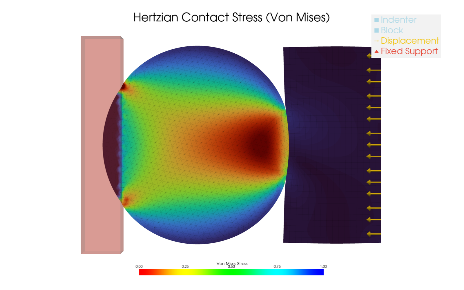
Fig. 61 Output of hertzian_contact.py: von Mises stress field on
the deformable indenter (circle) pressed against the
displaced block (right). Stress concentrates in a roughly
teardrop-shaped region inside the indenter, centered just
inboard of the contact patch — the classical Hertzian
subsurface stress distribution. The fixed left wall and
prescribed displacement arrows on the right block illustrate
the boundary setup.
Running it
cd examples/solid/hertzian_contact
python hertzian_contact.py    # writes hertzian_contact.png
Console output reports the contact-pressure distribution and the maximum displacement.
What’s next
Hyperelastic Beam (Neo-Hookean) — energy minimization recipe in isolation (no contact).
Plasticity (J2 with Isotropic Hardening) — a different non-quadratic energy driver (J2 plasticity), still with L-BFGS as the workhorse.