Quickstart
A complete 2D Poisson example: define a mesh, write the weak form in pure Python, apply Dirichlet boundary conditions, and solve. The full script is about 30 lines and runs in well under a second on a laptop CPU.
The problem
Solve the Poisson equation on the unit square \(\Omega = (0, 1)^2\) with homogeneous Dirichlet boundary conditions:
We pick \(f(x, y) = 2\pi^{2} \sin(\pi x)\sin(\pi y)\) so that the analytical solution is \(u(x, y) = \sin(\pi x)\sin(\pi y)\) — handy for sanity-checking the FEM result at the end.
The full script
import math
import torch
from tensormesh import ElementAssembler, NodeAssembler, Mesh, Condenser

# 1. Generate a triangular mesh of the unit square.
mesh = Mesh.gen_rectangle(chara_length=0.05)

# 2. Stiffness weak form: a(u, v) = ∫ ∇u · ∇v dΩ.
class LaplaceAssembler(ElementAssembler):
    def forward(self, gradu, gradv):
        return gradu @ gradv

# 3. Load weak form: l(v) = ∫ f v dΩ.
class SourceAssembler(NodeAssembler):
    def forward(self, v, f):
        return f * v

# 4. Source term f = 2π² sin(πx) sin(πy), evaluated at every mesh node.
x, y = mesh.points[:, 0], mesh.points[:, 1]
f_vals = 2 * math.pi**2 * torch.sin(math.pi * x) * torch.sin(math.pi * y)

# 5. Assemble the stiffness matrix K and load vector b.
K = LaplaceAssembler.from_mesh(mesh)()
b = SourceAssembler.from_mesh(mesh)(point_data={"f": f_vals})

# 6. Apply homogeneous Dirichlet BCs via static condensation, then solve.
condenser = Condenser(mesh.boundary_mask)
K_, b_ = condenser(K, b)
u = condenser.recover(K_.solve(b_))

# 7. Compare against the analytical solution and visualize.
u_exact = torch.sin(math.pi * x) * torch.sin(math.pi * y)
print(f"L2 error: {(u - u_exact).norm() / u_exact.norm():.3e}")

mesh.plot({"f": f_vals, "u_fem": u, "u_exact": u_exact}, save_path="poisson.png")
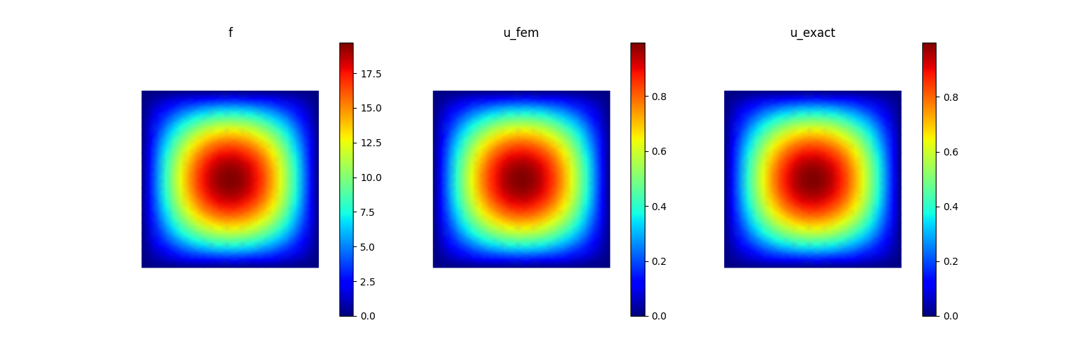
Running this script prints something like L2 error: 3.162e-03 and writes
a side-by-side plot of the source term f, the FEM solution, and the
analytical solution to poisson.png:
Note
Running on GPU. Add a single line after creating the mesh:
mesh = mesh.to("cuda")
Every tensor derived from mesh (assembled matrices, load vectors,
the condensed solve) then lives on the GPU automatically — including
f_vals here, since it is built from mesh.points. Only tensors
you construct independently of the mesh need to be moved over
explicitly, e.g. my_tensor = my_tensor.to(mesh.device).
Note
Built-in assemblers. The Laplace and source forms above are common
enough that TensorMesh ships ready-made versions
(LaplaceElementAssembler,
func_node_assembler(), and others), so you usually
don’t need to write them by hand. See Built-in assemblers for the
full catalogue.
Step by step
Mesh. Mesh stores nodes, cells, and any per-node /
per-cell data attached to them. gen_rectangle()
produces a triangular mesh of \((0, 1)^2\) with target element size
chara_length (smaller value → finer mesh).
Weak form. The two forward methods are the only things you write
that depend on the PDE — the library handles assembly. Inside
ElementAssembler, the arguments gradu, gradv
are the basis-function gradients already evaluated at every quadrature
point of every element; you return the integrand and the library does the
rest. NodeAssembler works the same way for vector-valued
integrands that depend on per-node data: pass the data via
point_data={...} and receive it as a keyword argument with the same
name.
Assembly. Assembler.from_mesh(mesh)() returns a
SparseMatrix (for ElementAssembler) or a torch
Tensor (for NodeAssembler). Internally everything is fused into a
single tensorized GPU kernel — no Python-level loop over elements.
Boundary conditions. Condenser applies Dirichlet
BCs by static condensation: condenser(K, b) returns a reduced system
on the interior DOFs only. After solving the reduced system,
recover() glues the inner solution back together
with the prescribed boundary values to produce a full-mesh solution.
Solve. solve() dispatches to a sparse solver
backend — by default SciPy on CPU and a torch-sla iterative solver on GPU.
See Sparse Solvers for the full backend matrix.
Convergence. The reported L2 error should be ≈ 3e-3 on the
default mesh; halve chara_length and the error drops by roughly a
factor of four — second-order convergence as expected for linear triangles.
What’s next
Verify Install — a smoke test that exercises CPU + (optional) GPU paths and reports which sparse-solver backends are wired up.
User Guide — meshes, custom forms, linear solvers, and differentiable workflows in depth.
Example Gallery — solid mechanics, wave propagation, inverse problems, and topology optimization.