Wave Equation

A single script, examples/wave/wave.py, solves the linear scalar
wave equation on the unit square with explicit central-difference
time stepping. It is the canonical hyperbolic counterpart to the
heat example in Diffusion.
The strong form is
with a multi-frequency Fourier-series initial condition from
WaveMultiFrequency and zero initial
velocity. The script runs at \(c = 2.0\),
\(\Delta t = 10^{-3}\), for 100 steps.
Central-difference time stepping
The standard discretization in time is
where \(M\) is the mass matrix and \(A\) is the Laplace stiffness. This is explicit in time — at each step we solve against a fixed mass matrix only, so factorize-once / back-sub-many is the right pattern.
The first step needs special treatment because \(U^{-1}\) is unknown; using the Taylor expansion \(U^{-1} \approx U^{0} - \Delta t\, V^{0}\) and the initial condition \(V^{0} = 0\) gives
TensorMesh setup
Two tiny assemblers (one for \(M\), one for \(A\)), one
Condenser for the homogeneous Dirichlet BC,
and a 15-line time loop. Note the small helper that scales a
SparseMatrix while keeping the
SparseMatrix type:
class AAssembler(ElementAssembler):
    def forward(self, gradu, gradv): return gradu @ gradv
class MAssembler(ElementAssembler):
    def forward(self, u, v):         return u * v

def scale_matrix(mat, s):
    return SparseMatrix(mat.edata * s, mat.row, mat.col, mat.shape)

mesh = Mesh.gen_rectangle(chara_length=0.01).to(device)
dataset = WaveMultiFrequency(K=16, c=c)

M = MAssembler.from_mesh(mesh, quadrature_order=2)()
A = AAssembler.from_mesh(mesh, quadrature_order=2)()
condenser = Condenser(mesh.boundary_mask)

u0 = dataset.initial_condition(mesh.points).to(device)
v0 = torch.zeros_like(u0)

# First step: 2 M U^1 = 2 M U^0 - dt^2 c^2 A U^0
cA = scale_matrix(A, c * c)
K  = scale_matrix(M, 2.0)
F  = -(dt*dt) * (cA @ u0) + 2.0 * (M @ u0) + (2.0 * dt) * (M @ v0)
K_, F_ = condenser(K, F)
U1 = condenser.recover(K_.solve(F_))
M_ = scale_matrix(K_, 0.5)            # K_ = 2 M_  →  M_ = K_/2

Us = [u0, U1]
for _ in range(n - 2):
    U_prev, U_curr = Us[-2], Us[-1]
    F  = 2.0*(M @ U_curr) - (M @ U_prev) - (dt*dt) * (cA @ U_curr)
    F_ = condenser.condense_rhs(F)
    U_ = M_.solve(F_)
    Us.append(condenser.recover(U_))
A few practical notes:
Stability. Central differences are conditionally stable — \(\Delta t \lesssim h / c\). The script’s choice (\(\Delta t = 10^{-3}\), \(h = 0.01\), \(c = 2\)) satisfies this comfortably.
Factorize once.
M_(the condensed mass matrix) is recovered from the first-step matrix and reused in every loop iteration; only the RHS changes.GPU-ready. The script picks
cudawhen available andmesh.to(device)moves the entire mesh + buffers in one call. Snapshots are moved back to CPU only at the end for visualization.
For a higher-order time integrator (Newmark, Runge-Kutta) drop in
ExplicitRungeKutta from
tensormesh.ode — see Time Integration.
Output of wave.py: FEM prediction (left) vs analytical
solution (right) for a multi-frequency standing wave on the unit
square. Phase and amplitude track the analytical reference
throughout the run; central differences preserve energy as long as
the CFL condition is satisfied.
Energy conservation
The undamped wave equation conserves the mechanical energy
with the velocity \(v = u_t\) taken as the centered difference of
the stored displacement history. wave.py evaluates this at every
step and writes wave_energy.png — a direct check on the time
stepping, since the central-difference scheme conserves a discrete
energy up to \(\mathcal{O}(\Delta t^2)\) whenever the CFL condition
holds.
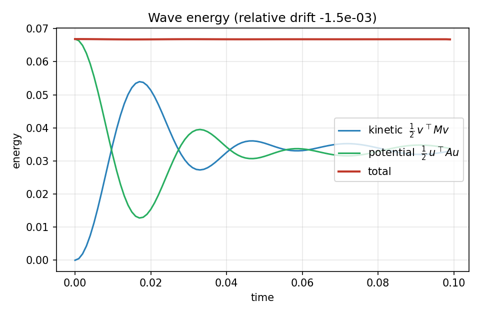
Fig. 41 Kinetic and potential energy exchange out of phase while the total (red) stays flat: the relative drift over the 100-step run is about \(1.5\times10^{-3}\). The motion starts as pure potential energy (zero initial velocity) and equipartitions as the standing wave develops.
Running the example
cd examples/wave
python wave.py        # writes wave.mp4 (FEM vs analytical) and wave_energy.png
What’s next
Phononic Crystals (Bloch-Floquet) — the frequency-domain cousin: Bloch-Floquet band structures and slab transmission for periodic acoustic media.
Time Integration — explicit and implicit-linear integrator classes.
Sparse Solvers — backend choice and the factorize-once / batched-solve recipes.
ML Datasets — the same wave equation, batched over 100 random initial conditions.
Diffusion — the parabolic counterpart with implicit Euler.