ML Datasets

Three scripts in examples/dataset/ generate large, ML-ready batches of PDE solutions for training neural operators (GAOT, FNO, Transolver, …). The recipe is the one outlined in Batched Workflows: same mesh, many right-hand sides, one factorization, multi-RHS back-substitution.

• poisson/poisson_dataset.py — 1000 steady-Poisson samples over random source fields, on a circular domain; the cleanest illustration of factor-once / back-sub-many.

• heat/heat_dataset.py — 1000 heat-equation samples, 100 timesteps, on an L-shaped domain.

• wave/wave_dataset.py — 1000 wave-equation samples, 100 timesteps, on a circular domain.

These three datasets are used in the GAOT paper (arXiv:2505.18781).

All three run on GPU when one is visible, fall back to SciPy on CPU, and benchmark the two paths against each other. The headline is how cheap this is: because the system matrix is factored only once and every sample — and, in the transient cases, every timestep — is just another right-hand side, generating a 1000-sample dataset costs barely more than a single solve. The timings below tell the story: 1000 steady Poisson solves in half a second, and 1000 transient runs of 100 steps each (a hundred thousand linear solves) in about ten seconds on a single GPU.

Poisson batched RHS — poisson_dataset.py

The steady-state warm-up: one stiffness matrix, many source fields. The script meshes a disk (radius \(0.5\), centered at \((0.5, 0.5)\), chara_length=0.008), draws 1000 multi-frequency Fourier source fields from PoissonMultiFrequency (K_modes=16), and solves all of them against a single assembled K.

The one Poisson-specific trick is the right-hand side. For a nodal source the load \(\int f\, v_i\,\mathrm{d}x\) equals \(M f\) with the mass matrix from the same quadrature, so the whole batch of loads is a single sparse matmul M @ f.T:

Listing 21 examples/dataset/poisson/poisson_dataset.py (essence)

from tensormesh import (LaplaceElementAssembler, MassElementAssembler,
                        Mesh, Condenser, NodeAssembler)
from tensormesh.dataset import PoissonMultiFrequency

class FAssembler(NodeAssembler):           # b_i = ∫ f v_i dx
    def forward(self, v, f):
        return v * f

mesh = Mesh.gen_circle(chara_length=0.008, cx=0.5, cy=0.5, r=0.5).to(device)

a  = torch.zeros((1000, 16, 16), device=device).uniform_(-1, 1)
eq = PoissonMultiFrequency(a=a)
f  = eq.source_term(mesh.points, domain="rectangle")   # [batch, n_points]

K = LaplaceElementAssembler.from_mesh(mesh)(mesh.points)
M = MassElementAssembler.from_mesh(mesh)(mesh.points)
b = M @ f.T                                            # [n_points, batch]

condenser = Condenser(mesh.boundary_mask,
                      torch.zeros(mesh.n_points, device=device))
K_, b_ = condenser(K, b)                               # [n_inner, batch]
u_     = K_.solve(b_)                                  # multi-RHS direct solve
u      = condenser.recover(u_).T                       # [batch, n_points]

The 2D RHS shape [n_inner, batch] is auto-routed to a direct solve: one factorization, batch back-substitutions. The script asserts M @ f.T matches the per-sample FAssembler load before solving, and cross-checks the GPU result against an independent CPU re-assembly.

On an NVIDIA RTX PRO 6000 (14478 DOFs total, 14145 inner, 1000 samples), all 1000 solves finish in half a second:

GPU solve (cuDSS, LDLᵀ):   0.51 s
CPU solve (SciPy, LU):     1.35 s
max |GPU − CPU|:           6.16e-17
speedup (CPU / GPU):       2.67×

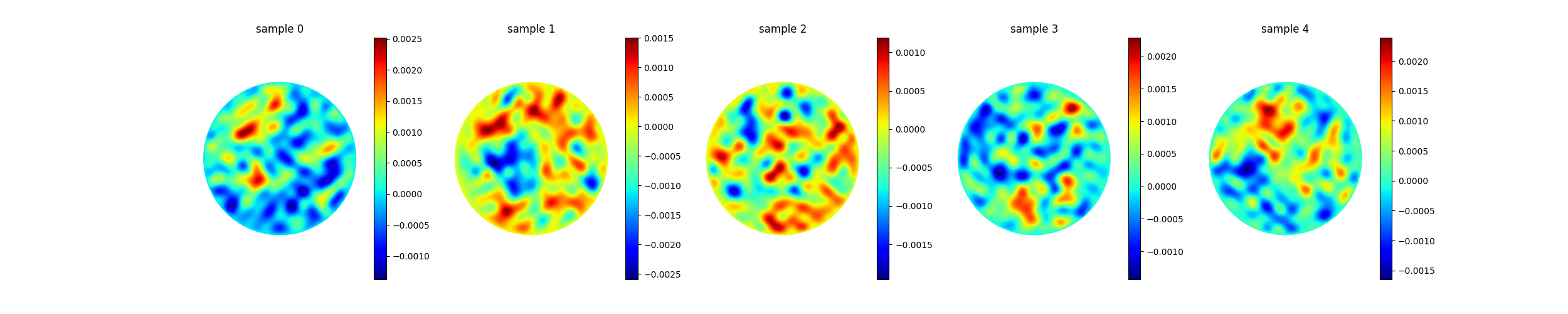
Fig. 57 Five representative samples from the generated dataset — the FEM Poisson solution on the disk for five random multi-frequency source fields. The script writes poisson_dataset.npz (solutions, sources, points, coefficients) alongside this figure.

Heat dataset on the L-shape — heat_dataset.py

Same backward-Euler scheme as Diffusion, but the time loop operates on a 2D snapshot U of shape [n_dofs, batch_size]:

Listing 22 examples/dataset/heat/heat_dataset.py

mesh = Mesh.gen_L(chara_length=0.008, element_type="tri").to(device)

batch_size, d, n = 1000, 16, 100
mus     = torch.rand((batch_size, d))            # random Fourier coeffs
dataset = HeatMultiFrequency(mu=mus)
u0s     = dataset.initial_condition(mesh.points)  # [batch_size, n_dofs]

M = MAssembler.from_mesh(mesh, quadrature_order=2)()
A = AAssembler.from_mesh(mesh, quadrature_order=2)()
condenser = Condenser(mesh.boundary_mask)

dt, D = 5e-5, 1.0
K_    = condenser(M + dt * D * D * A)[0]          # condense once

U = u0s.T.clone()                                  # [n_dofs, batch_size]
Us = [U]
for _ in range(n - 1):
    F  = M @ U                                     # [n_dofs, batch_size]
    F_ = condenser.condense_rhs(F)                 # [n_inner, batch_size]
    U_ = K_.solve(F_)                              # [n_inner, batch_size]
    U  = condenser.recover(U_)
    Us.append(U)

A few details that make the GPU path fast:

• F is a 2D tensor at every step; the sparse matrix-multiplication M @ U broadcasts over the batch axis on GPU.

• K_.solve(F_) with F_ shape [n_inner, batch_size] routes to torch-sla’s batched-RHS direct-solve path (K_ is a SparseMatrix, so .solve is the inherited torch_sla.SparseTensor.solve). On CPU this is SciPy’s LU; on GPU it is cuDSS — a Cholesky factorization here, since \(M + \Delta t\, D^2 A\) is SPD. One factorization is reused across all 1000 samples and all 100 timesteps.

• The L-shape is meshed at chara_length=0.008, giving about 14k DOFs — large enough that the batched direct solve dwarfs 1000 independent per-sample solves.

Output is a single .npz file with the full snapshot tensor:

heat_dataset.npz
    snapshots:  (100, 14052, 1000)   # n_steps × n_dofs × batch_size
    points:     (n_dofs, 2)
    mus:        (1000, 16)            # Fourier coefficients
    dt, D, n:   scalars

On an NVIDIA RTX PRO 6000 (14052 DOFs, 1000 samples, 100 steps):

GPU solve (cuDSS, Cholesky):   9.20 s
CPU solve (SciPy, LU):       123.26 s
max |GPU − CPU|:               9.09e-16
speedup (CPU / GPU):          13.39×

That GPU figure covers a hundred thousand linear solves (1000 samples × 100 timesteps), all sharing one factorization.

Animation of five samples from the generated heat dataset.

Wave dataset on the disk — wave_dataset.py

Same idea, central-difference scheme. The mesh is a circular domain (centered at \((0.5, 0.5)\), radius \(0.5\), chara_length=0.008), and the per-sample initial condition is parameterized by a 16×16 random Fourier-coefficient matrix \(a\):

batch_size, K, n = 1000, 16, 100
a = torch.zeros((batch_size, K, K)).uniform_(-1, 1)
dataset = WaveMultiFrequency(a=a, c=c)
u0s = dataset.initial_condition(mesh.points)        # [batch_size, n_dofs]

The [n_dofs, batch_size]-shaped time loop is identical in spirit to the heat case, with the wave-equation 3-term recurrence replacing the Euler step (see Wave Equation for the per-sample derivation). Output schema:

wave_dataset.npz
    snapshots:  (100, n_dofs, 1000)
    points:     (n_dofs, 2)
    a:          (1000, 16, 16)
    dt, c, n:   scalars

On an NVIDIA RTX PRO 6000 (14478 DOFs, 1000 samples, 100 steps):

GPU solve (cuDSS, LDLᵀ):    10.53 s
CPU solve (SciPy, LU):     175.51 s
max |GPU − CPU|:             1.03e-15
speedup (CPU / GPU):        16.68×

Animation of five samples from the generated wave dataset.

Running the examples

cd examples/dataset/poisson
python poisson_dataset.py              # writes poisson_dataset.{npz,png}

cd ../heat
python heat_dataset.py                 # writes heat_dataset.{npz,mp4}

cd ../wave
python wave_dataset.py                 # writes wave_dataset.{npz,mp4}

The GPU solve is auto-dispatched by torch-sla whenever CUDA is visible (cuDSS on the hardware above); see Sparse Solvers for the backend options.

What’s next

• Batched Workflows — the three axes of batching and when each one applies.

• Sparse Solvers — backend choice (cudss / cupy / scipy / pytorch / eigen) and how the direct solver is selected for batched RHS.