Time Integration¶

Transient problems — heat, wave, transient elasticity, phase-field dynamics — extend the static FEM pipeline with a time-stepping loop. Once the mass and stiffness matrices have been assembled, the semi-discrete weak form is just a system of ODEs in the nodal values

\[M\,\dot u(t) \;=\; A(t)\,u(t) \;+\; B(t), \qquad u(0) = u_0,\]

and the job of this chapter is to advance u from one time level to the next, accurately and stably, while keeping everything differentiable.

TensorMesh exposes two complementary styles:

A manual time-stepping loop. You assemble the time-stepped operator yourself, call Condenser once for the boundary conditions, and write a Python for loop that does one linear solve per step. Short, explicit, and the path of least resistance for a one-off problem.
The integrator classes in tensormesh.ode. You override forward(t, u) (explicit) or forward_M / forward_A / forward_B (linear-implicit), and call step(t, u, dt). Useful when you want a generic transient driver that lets you swap one scheme for another without rewriting the loop. The linear-implicit family composes with Condenser through three boundary-condition hooks (see Composing with boundary conditions), so static condensation of Dirichlet DOFs works inside the integrator too.

Both styles compose with torch.autograd, so gradients flow back through every step into initial conditions, material parameters, and boundary data alike (see Differentiability).

The integrator catalogue¶

tensormesh.ode ships three concrete schemes plus two extensible base classes:

Class	Order	Form	Use case
`ExplicitEuler`	1	\(\dot u = f(t, u)\)	Cheap explicit RHS; fine for non-stiff problems below the CFL.
`ImplicitLinearEuler`	1	\(M\dot u = A u + B\)	Heat / diffusion / stiff systems. Unconditionally stable.
`MidPointLinearEuler`	2	\(M\dot u = A u + B\)	Same family, second-order accurate (trapezoidal rule).
`ExplicitRungeKutta`	s-stage	\(\dot u = f(t, u)\)	Base class — supply your own Butcher tableau `(a, b)`.
`ImplicitLinearRungeKutta`	s-stage	\(M\dot u = A u + B\)	Same, for linear-implicit schemes.

For the explicit family you override forward(t, u) to return the right-hand side \(f(t, u)\). For the linear-implicit family you override three methods that return the operators at the current time:

class MyScheme(ImplicitLinearEuler):
    def forward_M(self, t):  return M_matrix    # SparseMatrix, Tensor, or scalar
    def forward_A(self, t):  return -K_matrix   # SparseMatrix, Tensor, or scalar
    def forward_B(self, t):  return 0.0         # Tensor or scalar

A scalar return is lifted to that multiple of the identity (or to a constant vector for B), so you can leave any of the three at their defaults of 1, 1, 0. Each call to step(t0, u0, dt) returns the new u advanced by one time step; u must be 1D ([D]), so flatten vector-valued problems before stepping.

Worked example 1: a scalar ODE¶

The integrator classes work on plain ODEs the same way they work on FEM systems — you just leave the operators as scalars. Take

\[\dot u(t) \;=\; -\lambda\,u(t), \qquad u(0) = 1, \qquad \lambda = \pi^{2},\]

whose exact solution is \(u(t) = e^{-\lambda t}\). Both ImplicitLinearEuler (first order) and MidPointLinearEuler (second order) accept a scalar M = 1 and A = -\lambda, so the driver is two short classes:

import torch
from tensormesh.ode import ImplicitLinearEuler, MidPointLinearEuler

class ScalarIE(ImplicitLinearEuler):
    def __init__(self, lam):
        super().__init__()
        self.lam = lam
    def forward_M(self, t): return 1.0
    def forward_A(self, t): return -self.lam
    def forward_B(self, t): return 0.0

class ScalarMP(MidPointLinearEuler):
    def __init__(self, lam):
        super().__init__()
        self.lam = lam
    def forward_M(self, t): return 1.0
    def forward_A(self, t): return -self.lam
    def forward_B(self, t): return 0.0

lam = torch.pi ** 2
u = torch.ones(1, dtype=torch.float64)
dt = 1e-3
integrator = ScalarMP(lam)
for k in range(50):
    u = integrator.step(k * dt, u, dt)

Running the same problem at decreasing \(\Delta t\) and measuring the error at \(T = 0.05\) produces the textbook order-1 and order-2 slopes:

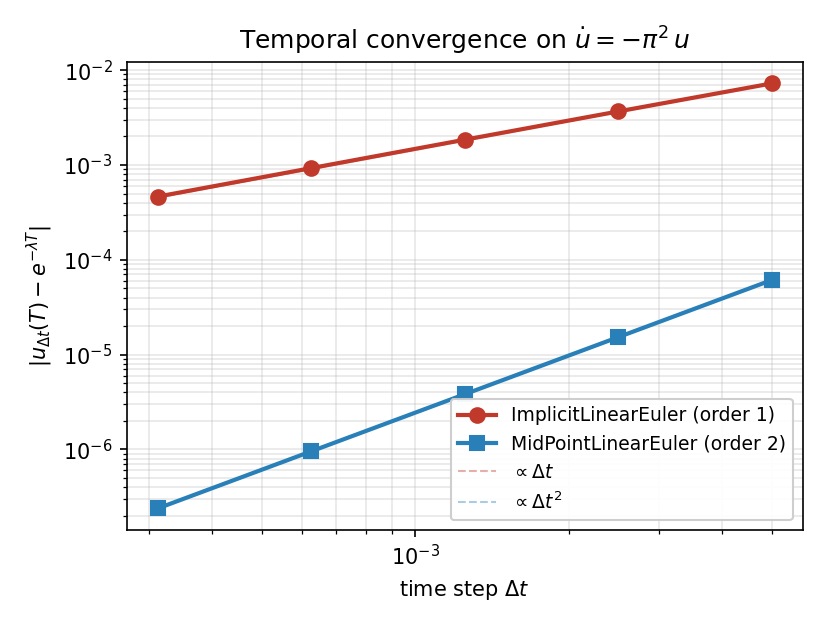
Temporal convergence on the scalar test ODE. — Fig. 11 Endpoint error vs `dt` for ImplicitLinearEuler and MidPointLinearEuler on \(\dot u = -\pi^{2}\,u\). Dashed reference lines have slopes 1 and 2.¶

The practical reading: spending a higher-order method buys you orders of magnitude in accuracy at the same step size — at dt = 5e-3 the midpoint rule already beats backward Euler by four orders of magnitude.

Worked example 2: 2D heat equation¶

For an FEM problem with Dirichlet boundaries, the manual loop is the cleanest pattern. Solve

\[\frac{\partial u}{\partial t} \;=\; \kappa\,\Delta u \quad \text{in } \Omega = (0, 1)^{2}, \qquad u = 0 \text{ on } \partial\Omega, \qquad u(x, y, 0) = \sin(\pi x)\,\sin(\pi y).\]

The semi-discrete form is \(M\dot u = -\kappa\,K\,u\), and one backward-Euler step gives the linear system

\[(M + \Delta t\,\kappa\,K)\,u^{n+1} \;=\; M\,u^{n}.\]

The full driver assembles M and K once, builds the time-stepped operator once, condenses it once, then loops:

import torch
from tensormesh import (Mesh, ElementAssembler,
                        MassElementAssembler, LaplaceElementAssembler,
                        Condenser)

mesh = Mesh.gen_rectangle(chara_length=0.025, order=1)
M = MassElementAssembler.from_mesh(mesh)().double()
K = LaplaceElementAssembler.from_mesh(mesh)().double()

kappa = 1.0
dt    = 5e-4

# Build the time-stepped operator once and condense it once.
A = M + dt * kappa * K
condenser = Condenser(mesh.boundary_mask)
A_in, _ = condenser(A, torch.zeros(mesh.n_points, dtype=torch.float64))

# Initial condition (already zero on the Dirichlet boundary).
x, y = mesh.points.double()[:, 0], mesh.points.double()[:, 1]
u = torch.sin(torch.pi * x) * torch.sin(torch.pi * y)

# Time stepping: each iteration is one mass-vector product,
# one RHS condensation, one back-substitution, one recovery.
snapshots = [u]
for _ in range(100):
    f       = M @ u
    f_in    = condenser.condense_rhs(f)
    u_in    = A_in.solve(f_in)
    u       = condenser.recover(u_in)
    snapshots.append(u)

The two ingredients that make this loop fast are (a) factorising the time-stepped operator only once — the per-step solve is a back-substitution through A_in — and (b) reusing the cached condenser layout via condense_rhs(). Together they turn what looks like an order-\(N^{3}\) problem into an order-\(N\) inner loop.

The solution decays exponentially as \(e^{-2\pi^{2}t}\):

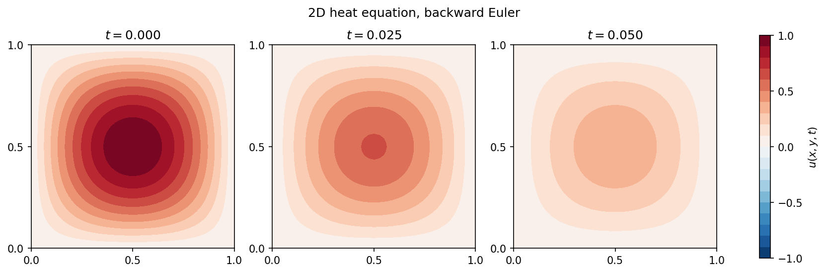
2D heat equation snapshots at three times. — Fig. 12 Snapshots of \(u(x, y, t)\) at \(t = 0\), \(t = T/2\), and \(t = T\) with \(T = 0.05\), backward Euler, \(\Delta t = 5\!\times\!10^{-4}\), characteristic mesh size \(h = 0.025\).¶

For an animated version, see the rendered heat.mp4 in the example gallery or under examples/diffusion/heat/ in the source tree.

Custom Butcher tableaux¶

The two RungeKutta base classes let you supply any Butcher tableau. To use the classical fourth-order explicit Runge-Kutta on \(\dot u = f(t, u)\):

import torch
from tensormesh.ode import ExplicitRungeKutta

a = torch.tensor([[0.,  0.,  0., 0.],
                  [0.5, 0.,  0., 0.],
                  [0.,  0.5, 0., 0.],
                  [0.,  0.,  1., 0.]])
b = torch.tensor([1/6, 1/3, 1/3, 1/6])

class MyRK4(ExplicitRungeKutta):
    def forward(self, t, u):
        return f(t, u)            # your problem-specific RHS

integrator = MyRK4(a, b)
for k in range(n_steps):
    u = integrator.step(k * dt, u, dt)

The class verifies that a is lower-triangular and that \(\sum_i b_i = 1\) (to within floating-point tolerance), so you catch transcription mistakes early. The same pattern with ImplicitLinearRungeKutta gives you diagonally-implicit or fully-implicit schemes — supply a non-zero diagonal and the class will assemble and solve the block stage system for you.

Composing with boundary conditions¶

Static condensation via Condenser (see Boundary Conditions) is the recommended way to enforce Dirichlet conditions in TensorMesh. Both time-integration styles support it; the only difference is where the three condenser calls go.

Mental model — what each solve is for

The two styles differ in what the linear solve is solving for, and that single fact dictates which Condenser calls are correct:

Manual loop → the unknown is the state \(u^{n+1}\). It takes the prescribed value \(u_o\) on the boundary, so you use the BC-value-aware calls (condense_rhs subtracts \(K_{io}\,u_o\); recover writes \(u_o\) back into the boundary slots).
Integrator hooks → the unknown is a stage slope \(k_i \approx \dot u\). A Dirichlet DOF is fixed in time, so \(\dot u = 0\) there whatever \(u_o\) is — the slope is zero on the boundary. You use the BC-value-free projections (restrict / prolong, which apply zero on the boundary in both directions).

The full-DOF state’s boundary value is carried along by \(u_0\) through the RK update \(u_{n+1} = u_0 + h\sum_i b_i k_i\); it is not re-imposed by the stage recovery.

At a glance, the same three operations map across the two styles like this — the rest of this section is just the detail behind each row:

Operation	Manual loop (state \(u\))	Integrator hooks (slope \(k\))
Condense the operator	`condenser(A)[0]` once, before the loop	`pre_solve_lhs(K)` → `condenser(K)[0]`
Project the RHS down	`condense_rhs(f)` — subtracts \(K_{io}\,u_o\)	`pre_solve_rhs(f)` → `restrict(f)` — no correction
Lift the solution back	`recover(u_in)` — writes \(u_o\) on the boundary	`recover_stage(k)` → `prolong(k)` — zero on the boundary

In a manual loop¶

The pattern is the same one used in Worked example 2:

call condenser(A, _) once, before the loop, to factorise the time-stepped operator on the interior DOFs;
call condenser.condense_rhs(f) every step to project the new RHS down to the interior;
call condenser.recover(u_in) after every solve to glue boundary values back in.

For time-varying boundary data, swap in the new values between steps with update_dirichlet() — the sparsity layout is cached and survives the update, so this call is cheap.

Through the integrator classes¶

ImplicitLinearRungeKutta (and its concrete subclasses) exposes three hooks that the step() method calls in the right places for static condensation to work end-to-end. Each hook is a no-op by default — override only the ones you need.

Hook	Called by `step()`	For `Condenser`-based BCs, return …
`pre_solve_lhs(K)`	once per `[i][j]` block of the stage system	the condensed inner block, `condenser(K)[0]`
`pre_solve_rhs(f)`	once per stage RHS	the restriction to inner DOFs, `condenser.restrict(f)` — not `condense_rhs(f)`: a stage slope is zero on the boundary by construction, so the \(-K_{io}\,u_o\) correction term in `condense_rhs` would over-apply the BC.
`recover_stage(k_i)`	once per stage, after the solve	the prolongation to full DOF with zero in the boundary slots, `condenser.prolong(k_i)` — not `recover`, which would write the Dirichlet value into the boundary slots and break the increment `u_{n+1} = u_n + h\sum_i b_i k_i`.

The fourth hook, post_solve(u), runs after the stage slopes have already been lifted and combined with \(u_0\), so u is always full-DOF when it sees you. Use it for things that act on the final state (clamping, normalisation, projection onto a manifold) rather than for boundary recovery.

The same three hooks cover multi-stage schemes unchanged: step() calls them once per stage (pre_solve_lhs once per [i][j] block), so a MidPointLinearEuler or a custom ImplicitLinearRungeKutta tableau wires up exactly like the backward-Euler example below.

Putting them together, a heat-equation driver becomes:

import torch
from tensormesh import (Mesh, MassElementAssembler,
                        LaplaceElementAssembler, Condenser)
from tensormesh.ode import ImplicitLinearEuler

class HeatStepper(ImplicitLinearEuler):
    """M du/dt = -kappa^2 K u, homogeneous Dirichlet via Condenser."""
    def __init__(self, M, K, kappa, condenser):
        super().__init__()
        self._M, self._A, self._cd = M, -kappa * kappa * K, condenser

    def forward_M(self, t):  return self._M
    def forward_A(self, t):  return self._A
    def forward_B(self, t):  return 0.0

    def pre_solve_lhs(self, K):  return self._cd(K)[0]       # condense stage block
    def pre_solve_rhs(self, f):  return self._cd.restrict(f)   # NOT condense_rhs
    def recover_stage(self, k):  return self._cd.prolong(k)    # NOT recover

# Same mesh and initial condition as Worked example 2.
mesh    = Mesh.gen_rectangle(chara_length=0.025, order=1)
M       = MassElementAssembler.from_mesh(mesh)().double()
K       = LaplaceElementAssembler.from_mesh(mesh)().double()
stepper = HeatStepper(M, K, kappa=1.0,
                      condenser=Condenser(mesh.boundary_mask))

x, y = mesh.points.double()[:, 0], mesh.points.double()[:, 1]
u    = torch.sin(torch.pi * x) * torch.sin(torch.pi * y)

dt = 5e-4
for step in range(100):
    u = stepper.step(step * dt, u, dt)

The examples/diffusion/heat/ directory ships both versions: heat.py (manual loop) and heat_ode.py (integrator class). They produce identical snapshots to machine precision — try them side by side.

Why `restrict` / `prolong` and not `condense_rhs` / `recover`¶

The two integrator hooks operate on the stage slope \(k_i \approx \dot u\), not on the state \(u\) itself. At a Dirichlet DOF \(u\) is held fixed in time, so \(\dot u = 0\) there regardless of the prescribed value. The two BC-value-aware methods on Condenser are designed for the state:

condense_rhs() subtracts \(K_{io}\,u_o\) from the inner RHS to account for the state’s prescribed boundary values;
recover() writes \(u_o\) into the boundary slots of the lifted solution.

Use those when condensing the state-space system (the manual loop). For stage slopes inside the integrator, use the BC-value-free projections restrict() and prolong(), which apply zero on the boundary in both directions. The difference vanishes for homogeneous Dirichlet (where \(u_o = 0\)), but matters as soon as the prescribed values are non-zero.

The bug is invisible under homogeneous Dirichlet

Mixing up the two pairs costs nothing when \(u_o = 0\), which is exactly why it slips through. Make it non-zero and it shows immediately. Take the heat problem above but hold the whole boundary at \(u_o = 1\) (interior starting at zero), backward Euler, \(\Delta t = 10^{-2}\), 40 steps, and measure against the manual state-space loop (condense_rhs / recover) as the reference:

Hook wiring	Interior error vs reference	Boundary (should stay `1.0`)
`restrict` + `prolong` (correct)	`4e-16` — machine precision	`1.0`
`condense_rhs` + `prolong`	`6e-3` — wrong interior	`1.0`
`restrict` + `recover`	`0.4` — drifts	`1.4` after 40 steps

condense_rhs subtracts a \(-K_{io}\,u_o\) term that the slope RHS never had, polluting the interior solution. recover writes \(u_o\) into the slope’s boundary slots, so the RK update adds \(h\,u_o\) to the boundary every step (here \(40 \times 10^{-2} \times 1 = 0.4\) of drift), breaking \(u_{n+1} = u_n + h\sum_i b_i k_i\). The restrict / prolong pair reproduces the manual loop to machine precision.

Explicit schemes¶

ExplicitRungeKutta has no linear solve and therefore no condensation hooks. The natural place for boundary conditions is inside the user-supplied forward(t, u): return \(f\) with f[boundary] = 0 and the update \(u_{n+1} = u_n + h \sum_i b_i k_i\) preserves \(u_{\text{boundary}}\) automatically.

import torch
from tensormesh import Mesh, MassElementAssembler, LaplaceElementAssembler
from tensormesh.ode import ExplicitEuler

mesh  = Mesh.gen_rectangle(chara_length=0.08, order=1)
M     = MassElementAssembler.from_mesh(mesh)().double()
K     = LaplaceElementAssembler.from_mesh(mesh)().double()
bmask = mesh.boundary_mask

class HeatExplicit(ExplicitEuler):
    """du/dt = M^{-1}(-kappa^2 K u), homogeneous Dirichlet."""
    def forward(self, t, u):
        f = M.solve(-(K @ u))     # semi-discrete RHS (lump M in production)
        f[bmask] = 0.0            # Dirichlet DOFs have zero time-derivative
        return f

x, y = mesh.points.double()[:, 0], mesh.points.double()[:, 1]
u    = torch.sin(torch.pi * x) * torch.sin(torch.pi * y)

dt = 5e-5                         # explicit -> small (CFL-limited) step
for step in range(50):
    u = HeatExplicit().step(step * dt, u, dt)

Because the boundary slope is forced to zero, u stays at its initial boundary value (0 here) for free. For time-varying Dirichlet data, write the analytical \(\dot u_{\text{b}}(t)\) into f[boundary] instead of zero, or overwrite the boundary slots of u between step() calls.

Differentiability¶

Every step is built on a differentiable solve (see Sparse Solvers), so back-propagation through a transient simulation is a no-op:

kappa = torch.tensor(1.0, requires_grad=True)
u     = run_heat_solver(mesh, kappa, dt=5e-4, n_steps=100)
loss  = (u - u_target).pow(2).sum()
loss.backward()
print(kappa.grad)            # gradient through 100 implicit solves

This is what makes transient inverse problems, parameter identification, and gradient-based PDE design straightforward in TensorMesh — see Differentiability for the longer story.

What’s next¶

Sparse Solvers — the solver behind every step.
Differentiability — backprop through a transient solve to optimise parameters or initial conditions.
Batched Workflows — batched initial conditions or parameters with the same transient driver.
Example Gallery — heat, wave, and transient elasticity demos with rendered animations.