Lid-Driven Cavity

The lid-driven cavity is the textbook benchmark for incompressible
Navier-Stokes solvers. The physics is simple — a box of fluid, the top
wall slides at unit speed, no-slip on the other walls, no body forces —
but at moderate Reynolds numbers it already exhibits a primary vortex
plus secondary corner eddies that any reasonable solver must reproduce.
Two scripts in examples/fluid/cavity/ run the steady-state problem
at \(\mathrm{Re} = 100\) with Taylor-Hood P2-P1 mixed
elements: cavity.py on a triangulated unit square and
cavity_3d.py on a tetrahedral unit cube. They share the same
scalar weak-form integrand — it is dimension-generic, so the 3D case
is essentially a mesh swap plus components=3.
Because the P2-P1 pair satisfies the discrete inf-sup (LBB) condition,
the plain Galerkin form is stable as-is: there are no SUPG/PSPG
stabilization terms and no tau parameter anywhere in these
scripts. The block bookkeeping (two fields, different orders,
different node sets) is owned by
MixedElementAssembler — see
Mixed Assembly for the machinery and
Taylor-Hood Stokes for the linear (Stokes) warm-up.
Problem
The strong form of the steady incompressible Navier-Stokes equations is
with \(\Omega = (0, 1)^d\), \(\mu = 1/\mathrm{Re}\), \(\rho = 1\), and boundary conditions
top lid (\(y = 1\)): \(\mathbf{u} = (1, 0, \dots)\) (moving wall)
other walls: \(\mathbf{u} = \mathbf{0}\) (no-slip)
one pressure DOF pinned to zero (the cavity is enclosed, so the pressure is only determined up to a constant).
Weak form and Picard linearization
Multiplying by test functions \((\mathbf{v}, q)\) and lagging the advecting velocity to the previous Picard iterate \(\mathbf{w} = \mathbf{u}^{n}\) gives the linearized mixed form: find \((\mathbf{u}, p)\) such that
for all \((\mathbf{v}, q)\). With Taylor-Hood spaces this needs no further ingredients, and the TensorMesh implementation is a direct transcription — two field declarations and the scalar integrand:
class NavierStokesAssembler(MixedElementAssembler):
    fields = [
        Field(trial="u", test="v", order=2, components=2),  # P2 velocity
        Field(trial="p", test="q", order=1),                # P1 pressure
    ]

    def __post_init__(self, rho=1.0, mu=0.01):
        self.rho = rho
        self.mu = mu

    def forward(self, gradu, p, v, gradv, q, w):
        convection = self.rho * (gradu @ w).dot(v)
        diffusion = self.mu * (gradu * gradv).sum()
        return convection + diffusion \
            - p * gradv.diagonal().sum() \
            - q * gradu.diagonal().sum()
gradu is the velocity Jacobian ([2, 2] in 2D, [3, 3] in
3D), so (gradu @ w).dot(v) is the convection term
\((\mathbf{w}\cdot\nabla)\mathbf{u}\cdot\mathbf{v}\) and
gradu.diagonal().sum() is the divergence. The lagged velocity
w is data (not a trial/test field), so the integrand stays
bilinear — the mixed assembler’s contract. Because the expression
never hard-codes the dimension, the same class serves 2D and 3D.
Picard iteration
Each iteration reassembles the matrix with the current velocity iterate and solves the linear saddle-point system:
mesh = Mesh.gen_rectangle(chara_length=1.0 / n_grid, order=2).double()
assembler = NavierStokesAssembler.from_mesh(mesh, rho=1.0, mu=1.0 / re)
layout = assembler.layout

bc_mask = layout.dof_mask("u", mesh.boundary_mask)   # no-slip everywhere
bc_mask[layout.dof_index("p", int(layout.node_ids("p")[0]))] = True  # pin

bc_val = torch.zeros(layout.n_dofs, dtype=torch.float64)
bc_val[layout.dof_mask("u", is_top, component=0)] = 1.0   # moving lid

condenser = Condenser(bc_mask, bc_val[bc_mask])
sol = torch.zeros(layout.n_dofs, dtype=torch.float64)
sol[bc_mask] = bc_val[bc_mask]

for i in range(max_iter):
    w = layout.split(sol)["u"]            # previous-iterate velocity
    K = assembler(point_data={"w": w})
    f = torch.zeros(layout.n_dofs, dtype=torch.float64)

    K_, f_ = condenser(K, f)
    sol = condenser.recover(K_.solve(f_))
    # ...convergence check on the relative update...
A few details that matter:
Block DOF layout. The solution vector stacks all velocity DOFs first, then the pressure DOFs.
layout.dof_mask/layout.dof_indexbuild boundary masks in that numbering, andlayout.split(sol)returns{"u": [n_u, 2], "p": [n_p]}— no hand-rolled index arithmetic anywhere.The lid mask. On the order-2 mesh the P2 velocity nodes are exactly the mesh points, so
point_data={"w": w}and node masks likeis_top = mesh.points[:, 1] > 1 - 1e-6apply directly.Quadrature. The default degree (
2 * max(order) = 4) is one shy of exact for the convection term — the standard, harmless choice; passquadrature_order=to integrate it exactly.
Picard converges geometrically at moderate Reynolds numbers — the relative update shrinks below \(10^{-4}\) in 8 iterations at Re = 100 on the default \(30 \times 30\) grid.
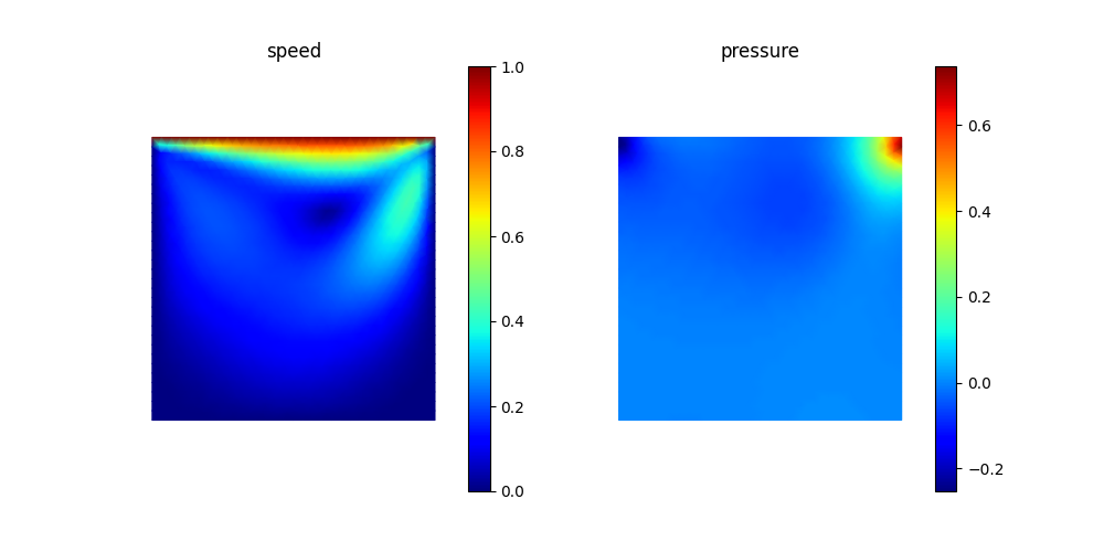
Fig. 67 Output of cavity.py at Re = 100 (Taylor-Hood P2-P1). Left:
speed magnitude \(\|u\|\) — the moving lid drags fluid into the
upper right, sweeping it down the right wall and forming the
primary vortex. Right: P1 pressure (prolonged to the P2 mesh points
for plotting), with the characteristic high-pressure spot in the
upper-right corner where the lid stagnates against the wall.
Going to 3D — cavity_3d.py
cavity_3d.py solves the same physics on a unit cube, and shows the
second way to obtain a Taylor-Hood pair: the tetrahedral mesh from
Mesh.gen_cube is linear, and the quadratic velocity space is
generated topologically by the mixed assembler (one extra DOF per
unique edge of the tet mesh) — no order-2 re-meshing. The field
declarations become
fields = [
    Field(trial="u", test="v", order=2, components=3),
    Field(trial="p", test="q", order=1),
]
and the forward integrand is byte-for-byte the one from 2D.
Because the velocity DOFs are no longer mesh points, the script uses
the layout’s topological helpers for boundary conditions and
post-processing:
x_u = layout.points("u")                                   # P2 node coordinates
is_boundary = layout.split(layout.boundary_mask("u"))["u"][:, 0]
is_top = is_boundary & (x_u[:, 1] > 1.0 - 1e-6)

bc_mask = layout.dof_mask("u", node_mask=is_boundary)      # no-slip walls
bc_val[layout.dof_mask("u", node_mask=is_top, component=0)] = 1.0

# Picard loop: the lagged velocity lives on the P2 field's own DOFs
K = assembler(field_data={"w": ("u", w)})

# post-processing: interpolate the P2 velocity back to mesh points
velocity = layout.prolong("u", layout.split(sol)["u"])
Note the two changes from 2D: boundary_mask finds the walls
topologically (facet incidence — no is_boundary point data
needed for the edge-generated nodes), and the lagged velocity enters
through field_data because it has no mesh-point representation.
At chara_length=0.1 the system has 24k DOFs (7.6k P2 velocity
nodes on 1.1k mesh points) and converges in 13 Picard iterations.
The output is volumetric: cavity_3d.vtu for ParaView plus a
\(z = 0.5\) mid-plane slice rendered via PyVista.
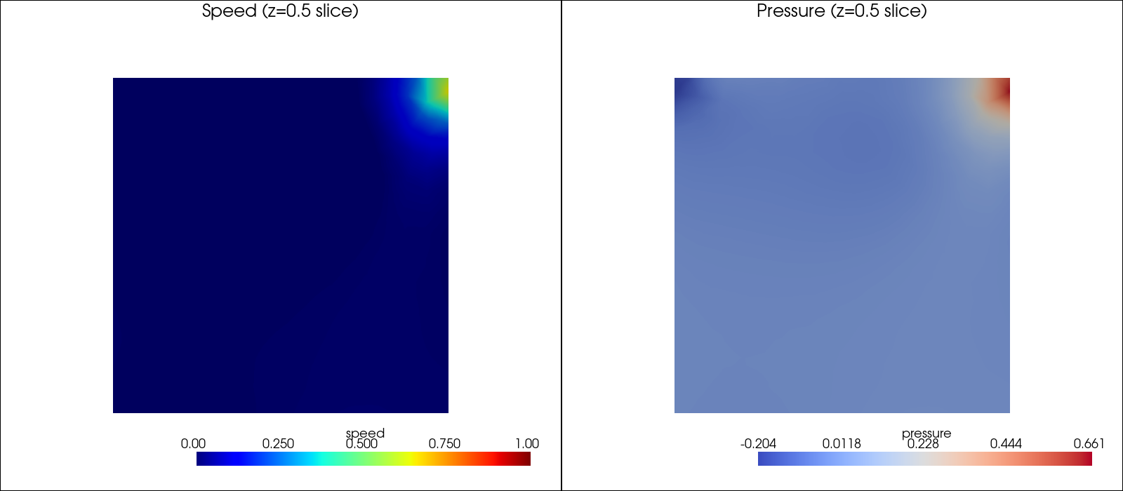
Fig. 68 Output of cavity_3d.py: speed magnitude (left) and pressure
(right) on the \(z=0.5\) mid-plane slice through the cube. The
flow pattern matches the 2D solution near the lid but decays toward
the front and back walls, so the mid-plane shows weaker
recirculation than the 2D benchmark.
Running it
cd examples/fluid/cavity
python cavity.py        # 2D, writes cavity_results.png
python cavity_3d.py     # 3D, writes cavity_3d.vtu + cavity_3d.png
Both converge in \(\lesssim 15\) Picard iterations at Re = 100 with the default resolutions.
What’s next
Taylor-Hood Stokes — the linear warm-up with a convergence study.
Cylinder Flow (Vortex Shedding) — the transient version: backward Euler,
forward_vectorload, vortex shedding.Rayleigh-Bénard Convection — add a third field (temperature) to the same block system.
Mixed Assembly — the mixed-assembly contract in full.