Basics & Visualization

Four short scripts in examples/basics/ that visualize the building blocks of FEM in TensorMesh: where interpolation nodes sit on the reference element, what the shape functions look like, how internal node numbering compares to Gmsh / VTK, and what the mesh generators produce. None of these scripts solve a PDE — they exist to make the underlying objects tangible and to sanity-check the conventions used elsewhere in the library.

If you are reading this page after the Elements and Quadrature user-guide page, treat these scripts as the picture book that goes with it.

Interpolation nodes

examples/basics/basis.py plots the spatial distribution of interpolation (Lagrange) nodes on the reference element for all seven element classes — Line, Triangle, Quadrilateral, Tetrahedron, Hexahedron, Pyramid, Prism — at orders 1 through 4. The driver is a one-liner per element class:

Listing 1 examples/basics/basis.py (essence)

from tensormesh.element import (
    Line, Triangle, Quadrilateral,
    Tetrahedron, Hexahedron, Pyramid, Prism,
)

for element in [Line, Triangle, Quadrilateral,
                Tetrahedron, Hexahedron, Pyramid, Prism]:
    for order in range(1, 5):
        basis = element.get_basis(order)   # [n_basis, dim]
        # …scatter basis on the reference element…

The number of basis points grows quickly with order: \((p+1)^d\) for tensor elements, \(\binom{p+d}{d}\) for simplex elements. Knowing where they sit is the first sanity check when something goes wrong with a higher-order solve.

The seven panels below show the Lagrange-node layout for every supported element class at orders 1–4. Each panel reads left-to-right by order; node indices match the internal element.get_basis(order) ordering.

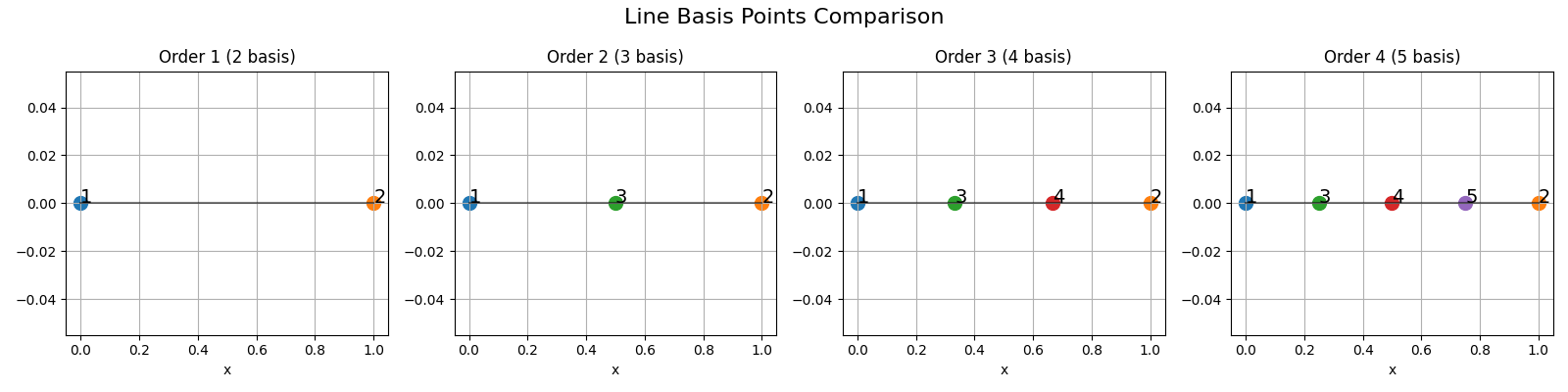
Fig. 19 Line element — lexicographic ordering on \([0, 1]\).

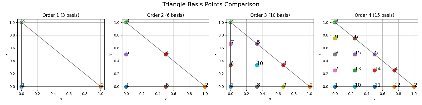
Fig. 20 Triangle element — simplex ordering with vertex nodes first, then edge nodes, then interior nodes.

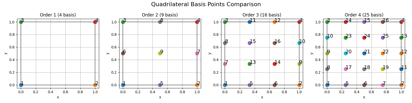
Fig. 21 Quadrilateral element — tensor-product Lagrange nodes.

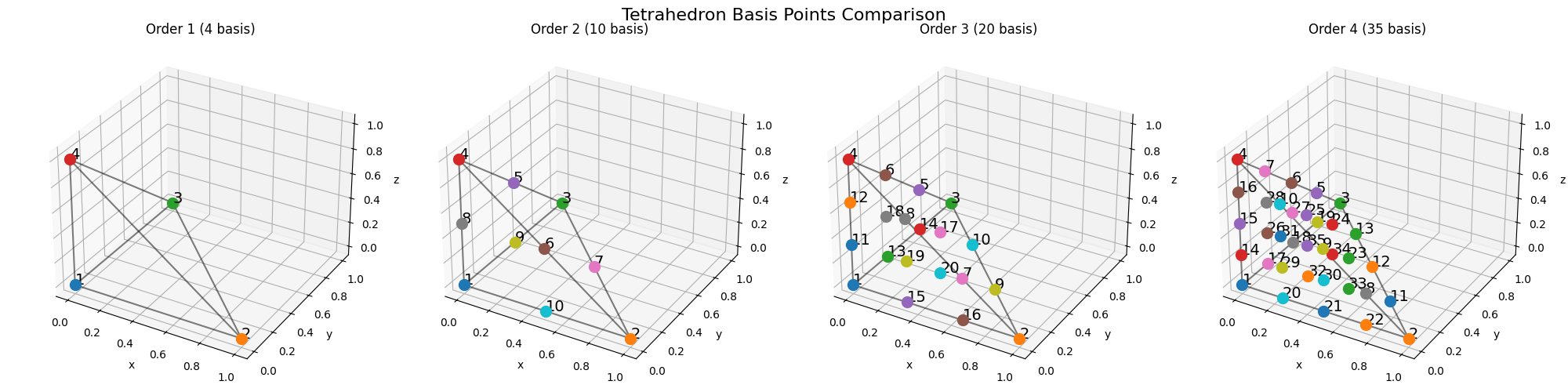
Fig. 22 Tetrahedron element — 3D simplex.

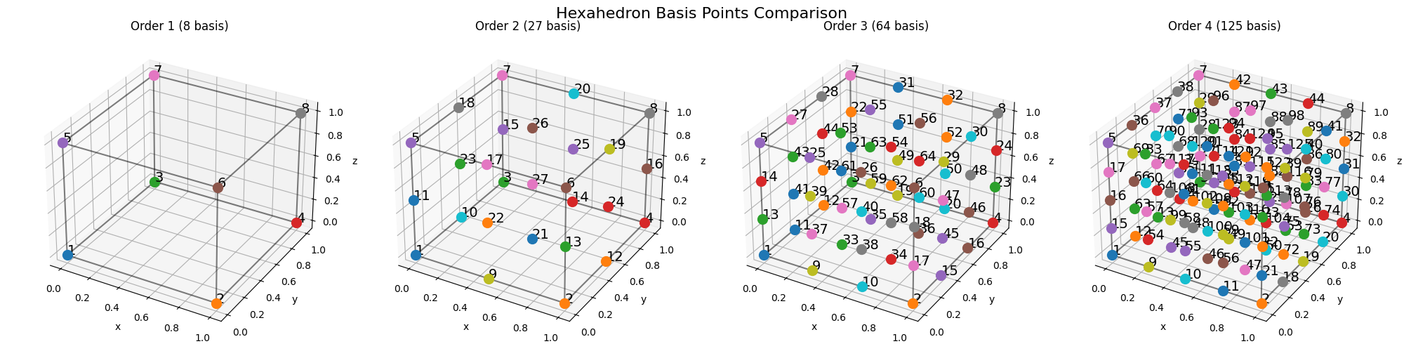
Fig. 23 Hexahedron element — 3D tensor product.

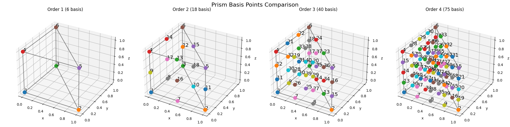
Fig. 24 Prism (wedge) element — triangle \(\times\) line.

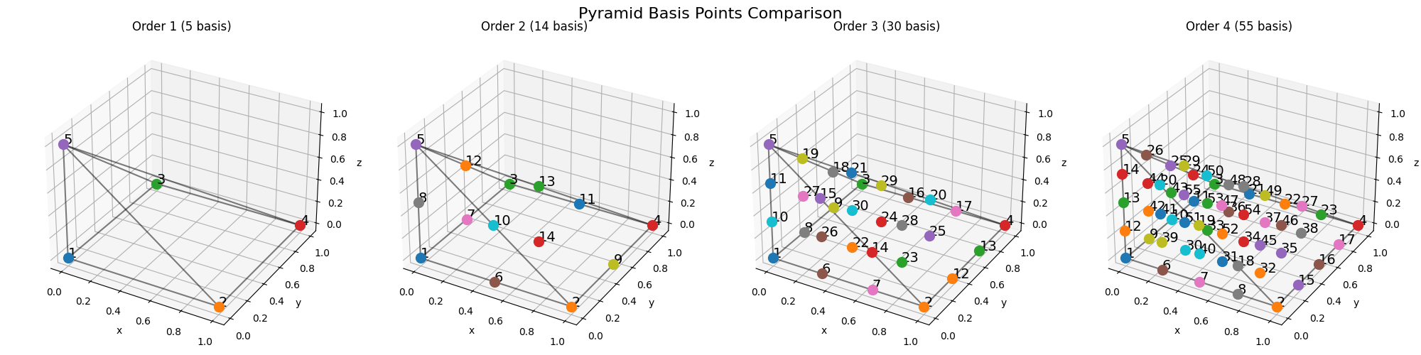
Fig. 25 Pyramid element — square base, apex at the top.

Shape functions

examples/basics/basis_fn.py plots the polynomial shape functions themselves. For 1D elements they appear as curves on \([-1,1]\); for 2D elements as 3D surfaces on the reference triangle or square; for 3D elements one figure per order with a slice through the volume.

The script uses element.get_basis_fns(order), the same call ElementAssembler makes during assembly. If a shape function looks wrong here, it is wrong in your assembled matrix too.

In principle get_basis_fns accepts arbitrary polynomial order — there is no hard cap baked into the API. The figures below show 1D and 2D shape functions at orders 1–3 (plus the full composite view) and 3D shape functions at order 1; higher 3D orders are equally available, they are simply omitted here for space.

Note

Although arbitrary orders are supported, very high orders (in practice \(\geq 4\) for some element classes) are evaluated through a Vandermonde matrix that becomes increasingly ill-conditioned with order. The script may print a numerical warning in that regime. The returned values are still usable — but if you see those warnings during a real solve, drop to a lower order or switch to a different element class. For most FEM workloads orders 1–3 are the sweet spot.

1D and 2D shape functions

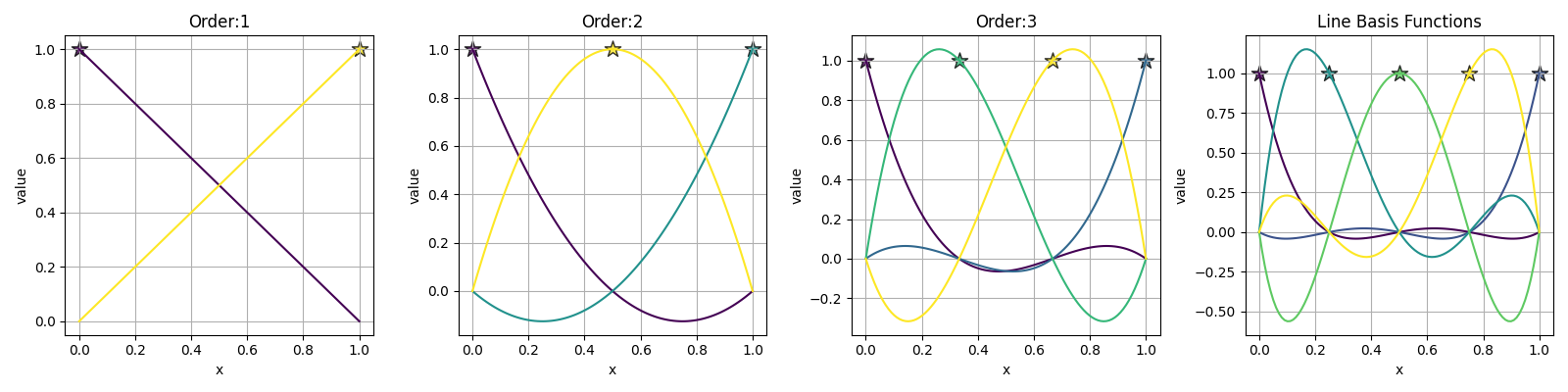
Fig. 26 Line shape functions at orders 1–3, plus a composite view of the highest order. Stars mark the interpolation nodes.

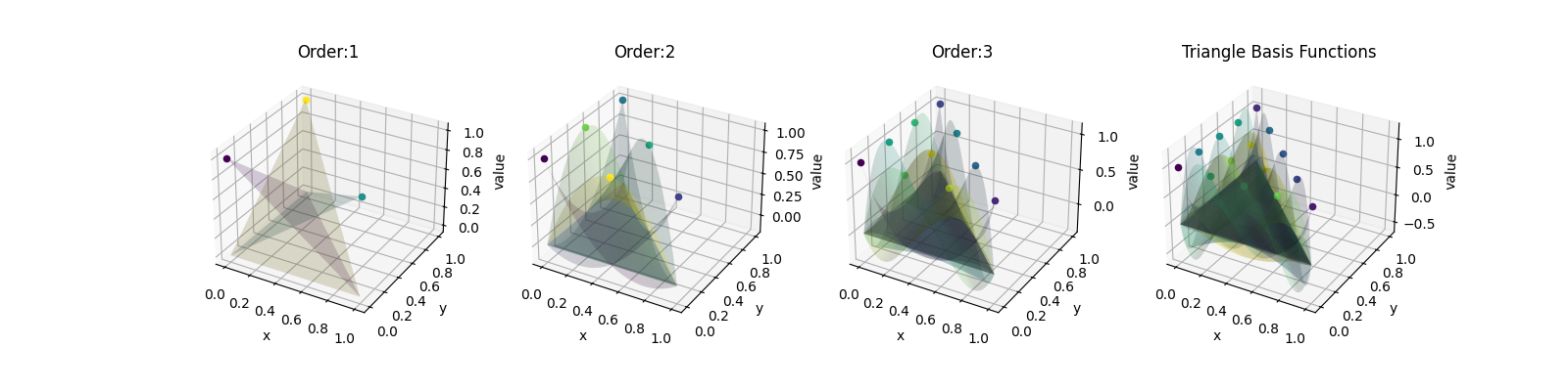
Fig. 27 Triangle shape functions plotted as 3D surfaces over the reference triangle.

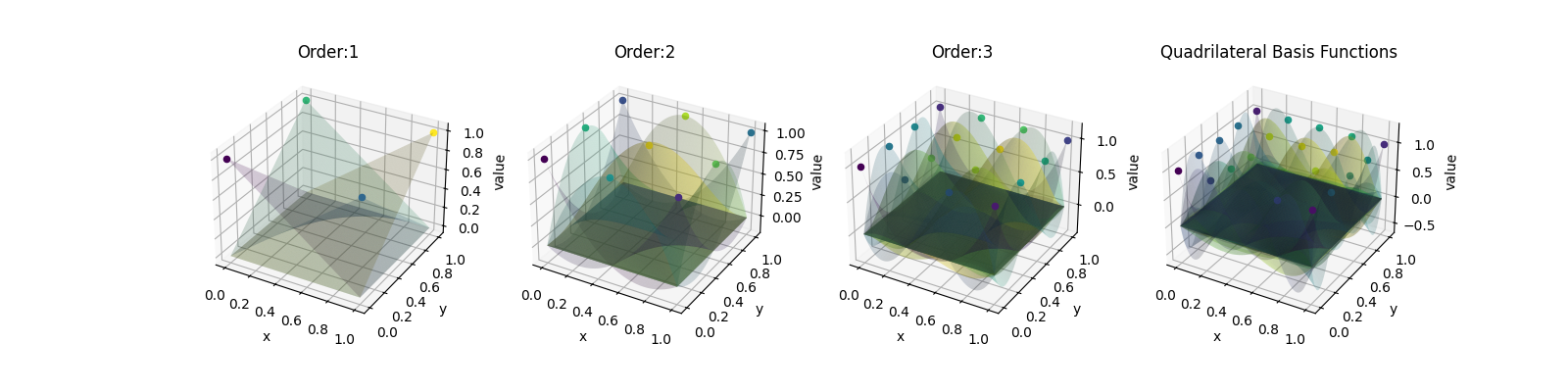
Fig. 28 Quadrilateral shape functions on the reference square.

3D shape functions (order 1)

For 3D elements the script renders one volumetric figure per element / order combination; only the order-1 panels are shown below. The full set (including orders 2–4) lands in examples/basics/output/<element>/<order>.png after running the script.

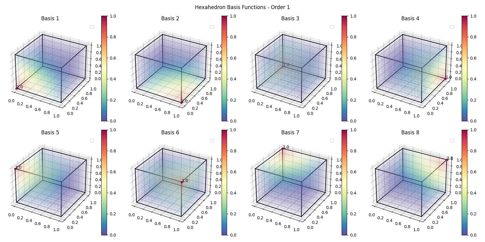
Fig. 29 Hexahedron order-1 shape functions — eight trilinear basis functions, one per vertex.

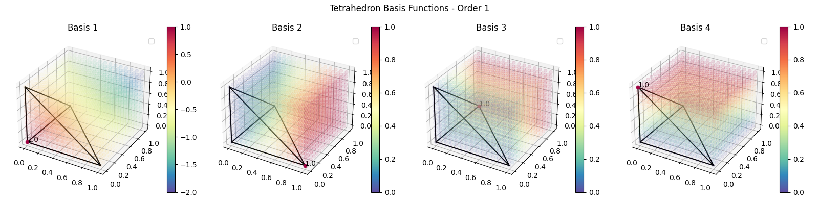
Fig. 30 Tetrahedron order-1 shape functions — four barycentric coordinates.

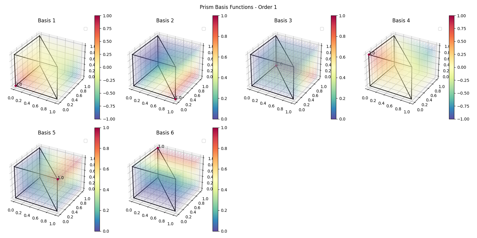
Fig. 31 Prism order-1 shape functions — six basis functions, one per vertex of the triangular prism.

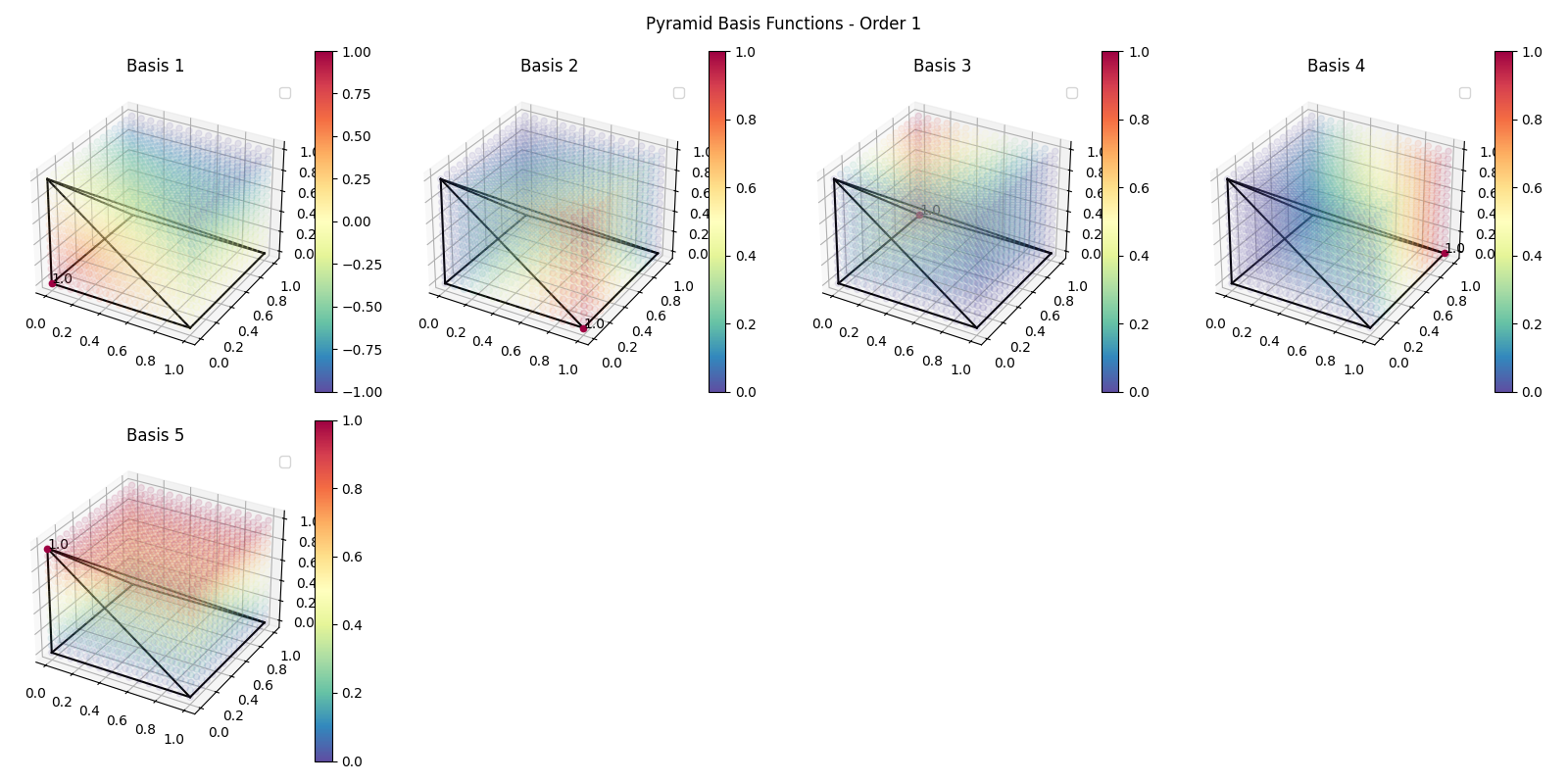
Fig. 32 Pyramid order-1 shape functions — five basis functions, one per vertex.

Gmsh / VTK ↔ TensorMesh node ordering

examples/basics/element_gallery.py puts TensorMesh’s internal node numbering side-by-side with the Gmsh / VTK convention, for 2D and 3D elements at orders 2–4. The output is a two-row plot per element type: top row is the TensorMesh / FEniCS-style ordering; bottom row is the Gmsh / VTK ordering.

This is the visual companion to the reorder=True story in Meshes: when you load a Gmsh .msh or write a VTU through meshio, TensorMesh applies the inverse permutation returned by element.get_gmsh_permutation(order) so internal connectivity always uses the same convention. If you ever question which numbering a particular array is in, this script makes it obvious.

Four representative comparisons are shown below — one per element family. The remaining element types (line, prism, pyramid) follow the same two-row layout; the full set lives in examples/basics/output/element_gallery/.

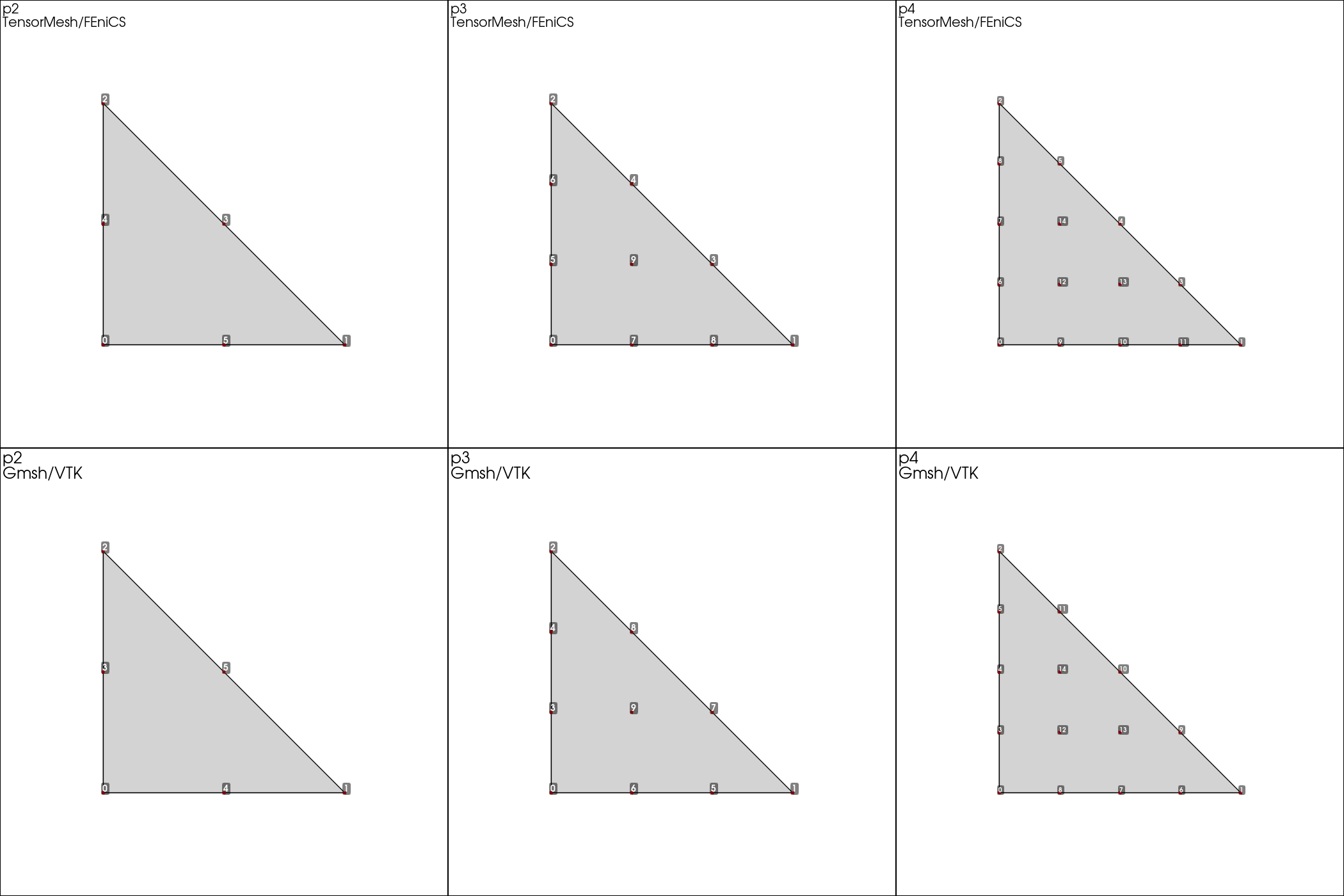
Fig. 33 Triangle — top row: TensorMesh / FEniCS ordering; bottom row: Gmsh / VTK ordering.

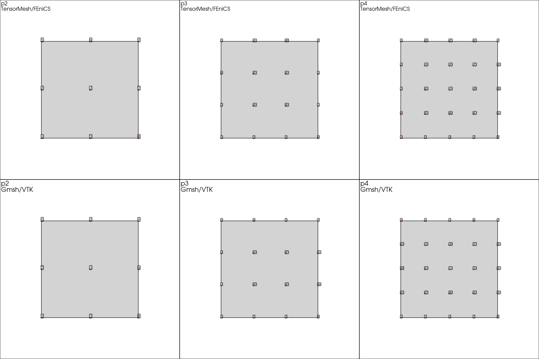
Fig. 34 Quadrilateral — note that the TensorMesh layout is lexicographic, while Gmsh’s order-3 / order-4 quad layouts spiral around the boundary.

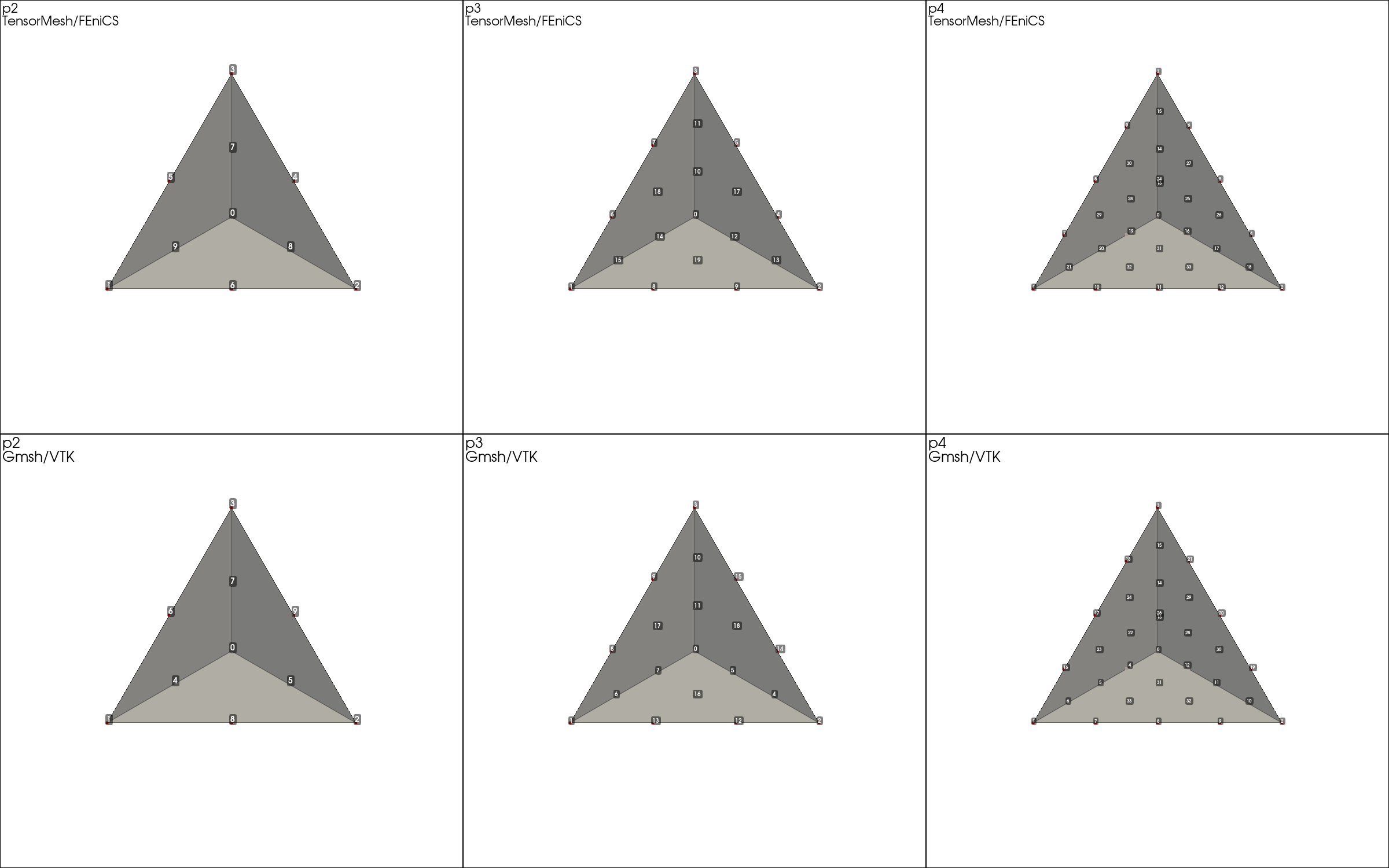
Fig. 35 Tetrahedron — vertex / edge / face / interior groupings are preserved across both orderings, only the indices within each group differ.

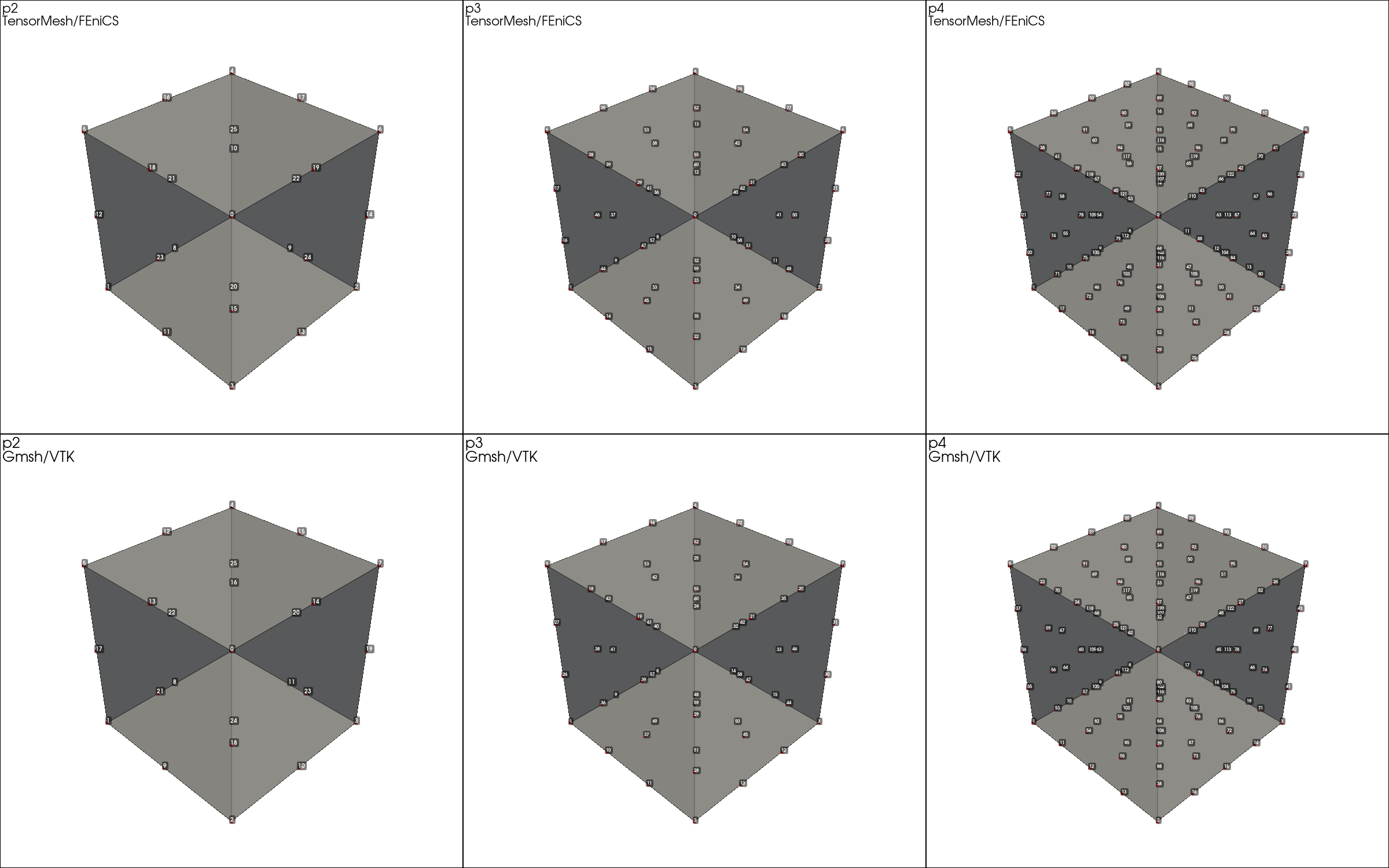
Fig. 36 Hexahedron — the largest discrepancy in the gallery, since Gmsh’s hex ordering walks along edges while TensorMesh’s is plain lexicographic.

Mesh generation gallery

examples/basics/plot_mesh.py is the picture catalog of what TensorMesh’s mesh tools can produce, plus a few visualization helpers from tensormesh.visualization:

• Built-in primitives — rectangle (triangle and quadrilateral), cube (tetrahedral and hexahedral, the latter with quadratic basis), and a unit disk via MeshGen.

• Hybrid meshes — half the rectangle is meshed with triangles, the other half with quadrilaterals, and a circular hole is punched in the interface. mesh.cells is a BufferDict keyed by element type, so all assemblers iterate over both element types automatically.

• Adjacency graphs — node-to-node and element-to-element connectivity drawn over the mesh, in 2D and 3D. Useful for debugging coloring and partitioning algorithms (see Distributed FEM).

• Field visualization — scalar fields painted as nodal values (interpolated to the mesh) or as per-element constants.

A representative snippet for the hybrid mesh:

Listing 2 examples/basics/plot_mesh.py (essence)

import tensormesh as tm

mesh_gen = tm.MeshGen(element_type=None, chara_length=0.1, order=2)
mesh_gen.add_rectangle(0,   0, 0.5, 1, element="tri")
mesh_gen.add_rectangle(0.5, 0, 0.5, 1, element="quad")
mesh_gen.remove_circle(0.5, 0.5, 0.1)
mesh = mesh_gen.gen()
mesh.plot(save_path="output/hybrid_mesh2d.png")

The corresponding 3D scripts use dimension=3 plus add_cube / remove_sphere for CSG.

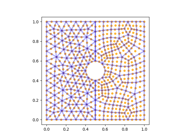
Fig. 37 Hybrid 2D mesh produced by the snippet above: order-2 triangles on the left, order-2 quadrilaterals on the right, and a circular hole at the interface. Orange dots are the interpolation nodes (including mid-edge nodes from the order-2 elements).

Running the scripts

All four are standalone:

cd examples/basics
python basis.py
python basis_fn.py
python element_gallery.py
python plot_mesh.py

Outputs land under examples/basics/output/ — one PNG per script or, for the multi-element scripts, one PNG per (element, order) combination.

What’s next

• Elements and Quadrature — the element zoo and the basis / quadrature interface these scripts call into.

• Meshes — meshing API, reorder=True, and per-node / per-element data.

• Poisson Equation — first PDE solve, using the same Mesh objects you just learned to build.