Rayleigh-Bénard Convection
The Rayleigh-Bénard problem couples incompressible fluid flow with
heat transport: a horizontal cavity heated from below, cooled from
above, develops convective rolls once the buoyancy force exceeds
the dissipative effects of viscosity and thermal diffusion. The
script examples/fluid/rayleigh_benard/rayleigh_benard.py solves
the Boussinesq approximation in a 2:1 aspect-ratio rectangular
cavity at a configurable Rayleigh number.
This is the gallery’s three-field mixed example: Taylor-Hood
P2-P1 velocity/pressure plus a P2 temperature, all declared on
one MixedElementAssembler. The buoyancy
coupling and the energy equation are just more terms of the same
scalar integrand — no per-node block stamping, no stabilization.
Problem
The transient Boussinesq equations,
on \(\Omega = [0, 2] \times [0, 1]\), with
velocity: no-slip on all walls,
temperature: \(T = 1\) on the bottom (\(y = 0\)), \(T = 0\) on the top (\(y = 1\)), no-flux on the side walls,
one pressure DOF pinned (enclosed cavity).
The Rayleigh number
controls the regime: below \(\mathrm{Ra}_c \approx 1708\) heat transfer is purely conductive; above it convective rolls appear. The script defaults to \(\mathrm{Ra} = 2 \times 10^4\) (\(\mathrm{Pr} = 1\)), comfortably in the steady-convective regime.
Why march in time? The conductive state (linear temperature, zero velocity) is a steady solution at every Rayleigh number — a steady solver started from rest simply converges to it. Above \(\mathrm{Ra}_c\) that state is unstable, so the script perturbs the conductive profile slightly and integrates backward Euler in time: the instability grows physically into convection rolls, and the run stops when the solution stops changing.
Three fields, one integrand
The unknowns are declared as three fields — trial names (u, p,
T), test names (v, q, s). Every term of the coupled weak form
pairs one trial factor with one test factor, so the whole system is
one bilinear integrand:
class RayleighBenardAssembler(MixedElementAssembler):
    fields = [
        Field(trial="u", test="v", order=2, components=2),  # P2 velocity
        Field(trial="p", test="q", order=1),                # P1 pressure
        Field(trial="T", test="s", order=2),                # P2 temperature
    ]

    def __post_init__(self, rho=1.0, mu=0.1, kappa=0.1,
                      g=10.0, beta=1.0, dt=1e-2):
        self.rho, self.mu, self.kappa = rho, mu, kappa
        self.g, self.beta, self.dt = g, beta, dt

    def forward(self, u, gradu, p, T, gradT, v, gradv, q, s, grads, w):
        momentum = self.rho / self.dt * u.dot(v) \
            + self.rho * (gradu @ w).dot(v) \
            + self.mu * (gradu * gradv).sum() \
            - p * gradv.diagonal().sum() \
            - self.rho * self.g * self.beta * T * v[1]   # buoyancy
        continuity = -q * gradu.diagonal().sum()
        energy = T * s / self.dt \
            + w.dot(gradT) * s \
            + self.kappa * gradT.dot(grads)
        return momentum + continuity + energy

    def forward_vector(self, v, s, uprev, Tprev):
        return self.rho / self.dt * uprev.dot(v) + Tprev * s / self.dt
Two couplings deserve a closer look:
Buoyancy
- rho g beta T v[1]pairs the trial temperature with the vertical velocity test function — an off-diagonal \((v, T)\) block that the mixed assembler extracts automatically. Temperature therefore feeds back into momentum fully implicitly; only the advecting velocitywis lagged (Picard).Energy transport
w.dot(gradT) * s + kappa *
gradT.dot(grads)
is a scalar advection-diffusion equation riding in the same matrix, with the same laggedw.
Time marching to the attractor
Each backward-Euler step assembles the matrix with the current velocity and the load vector with the previous fields, both through the same assembler:
T0 = (1.0 - y) + 0.01 * torch.sin(math.pi * x / 2) * torch.sin(math.pi * y)
sol = layout.cat(u=0.0, p=0.0, T=T0)

for step in range(n_steps):
    fields = layout.split(sol)
    K = assembler(point_data={"w": fields["u"]})
    f = assembler.assemble_vector(
        point_data={"uprev": fields["u"], "Tprev": fields["T"]})
    K_, f_ = condenser(K, f)
    sol = condenser.recover(K_.solve(f_))
    # stop when the per-step relative update stalls (steady state)
On the order-2 mesh both P2 fields (velocity and temperature) live
on the mesh points, so the lagged data goes through plain
point_data and the final fields plot directly.
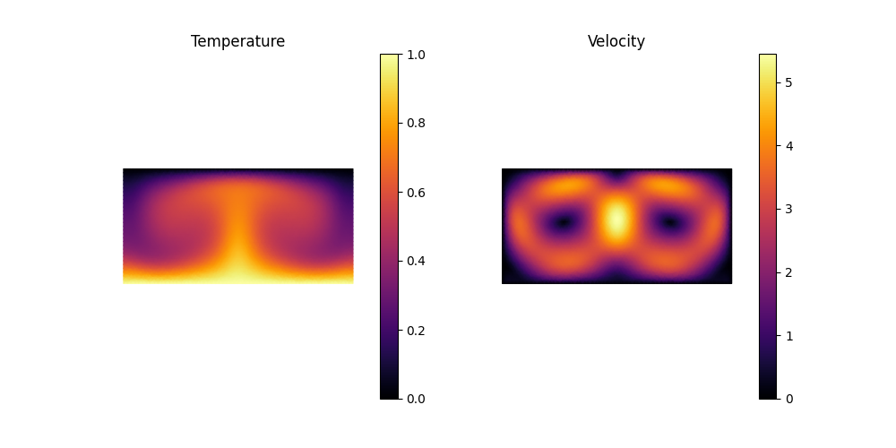
Fig. 70 Output of rayleigh_benard.py. Left: temperature field —
the warm bottom wall sends rising plumes that split at the cold
top into cool downward plumes. Right: velocity magnitude —
counter-rotating convection rolls, with peak speeds along the
rising / sinking columns and stagnation at the roll centers.
Running it
cd examples/fluid/rayleigh_benard
python rayleigh_benard.py     # writes rayleigh_benard.png
Edit the ra= argument to sweep the Rayleigh number; values much
above \(10^5\) become unsteady and need a finer mesh and
smaller time step.
What’s next
Lid-Driven Cavity — the same Picard recipe without temperature coupling.
Taylor-Green Vortex (Convergence Study) — a transient incompressible flow with an exact solution for verification.
Diffusion — the heat equation in isolation.
Mixed Assembly — declaring fields and writing multi-field integrands.