Taylor-Hood Stokes

The entry point to mixed assembly: the script examples/fluid/stokes_taylor_hood/stokes_taylor_hood.py solves a manufactured incompressible Stokes problem on the unit square with the classic Taylor-Hood P2-P1 pair, verifies the solution against the exact fields, and runs an h-refinement convergence study. If you are new to MixedElementAssembler, start here — the cavity, cylinder and Rayleigh-Bénard examples all build on this pattern. The concepts are covered in Mixed Assembly.

Problem

The Stokes equations with a body force,

\[-\mu\, \Delta \mathbf{u} + \nabla p = \mathbf{f} \quad \text{in } \Omega = (0,1)^2, \qquad \nabla \cdot \mathbf{u} = 0,\]

with \(\mathbf{f}\) manufactured from a divergence-free exact velocity (derived from the stream function \(\psi = \sin^2(\pi x)\,\sin^2(\pi y)\)) and the exact pressure \(p = \sin(\pi x)\cos(\pi y)\). Dirichlet data on the boundary is the exact velocity; one pressure DOF is pinned to the exact value to fix the constant null space.

Because the exact pressure is not in the P1 space and the exact velocity is not in the P2 space, the discrete errors are genuine approximation errors — ideal for measuring convergence rates.

The mixed weak form

Multiply by test functions \((\mathbf{v}, q)\) and integrate by parts:

\[\int_\Omega \mu\,\nabla\mathbf{u} : \nabla\mathbf{v}\,\mathrm{d}x - \int_\Omega p\,(\nabla\cdot\mathbf{v})\,\mathrm{d}x - \int_\Omega q\,(\nabla\cdot\mathbf{u})\,\mathrm{d}x \;=\; \int_\Omega \mathbf{f}\cdot\mathbf{v}\,\mathrm{d}x .\]

In TensorMesh this is the code — two field declarations and a four-line integrand:

Listing 18 examples/fluid/stokes_taylor_hood/stokes_taylor_hood.py (essence)

class StokesAssembler(MixedElementAssembler):
    fields = [
        Field(trial="u", test="v", order=2, components=2),  # P2 velocity
        Field(trial="p", test="q", order=1),                # P1 pressure
    ]

    def __post_init__(self, mu=1.0):
        self.mu = mu

    def forward(self, gradu, p, gradv, q):
        div_u = gradu.diagonal().sum()
        div_v = gradv.diagonal().sum()
        return self.mu * (gradu * gradv).sum() - p * div_v - q * div_u

gradu is the \(2 \times 2\) velocity Jacobian, so (gradu * gradv).sum() is \(\nabla\mathbf{u}:\nabla\mathbf{v}\) and gradu.diagonal().sum() is \(\nabla\cdot\mathbf{u}\). Trial fields (u, p) index matrix columns, test fields (v, q) rows. The P2-P1 pair satisfies the discrete inf-sup (LBB) condition, so no stabilization terms appear anywhere.

Boundary conditions via the layout

assembler.layout translates “field, nodes, component” into global block-DOF indices, so the saddle-point structure never leaks into the BC code:

mesh = Mesh.gen_rectangle(chara_length=h, order=2, element_type="tri").double()
assembler = StokesAssembler.from_mesh(mesh, quadrature_order=7, mu=mu)
layout = assembler.layout

bc_mask = layout.dof_mask("u", mesh.boundary_mask)          # velocity Dirichlet
pressure_pin = layout.dof_index("p", int(layout.node_ids("p")[0]))
bc_mask[pressure_pin] = True

bc_val = torch.zeros(layout.n_dofs, dtype=torch.float64)
bc_val[layout.dof_mask("u")] = exact_velocity(mesh.points).reshape(-1)
bc_val[pressure_pin] = exact_pressure(layout.points("p"))[0]

condenser = Condenser(bc_mask, bc_val[bc_mask])

The body force is assembled with a plain NodeAssembler on the velocity space (the order-2 mesh points are the P2 nodes) and placed into the block vector with layout.cat:

f = layout.cat(u=body_rhs, p=0.0)
K = assembler()

K_inner, f_inner = condenser(K, f)
sol = condenser.recover(K_inner.solve(f_inner))
fields = layout.split(sol)          # {"u": [n_u, 2], "p": [n_p]}

Convergence study

Taylor-Hood theory promises \(O(h^2)\) in the velocity \(H^1\) norm and \(O(h^2)\) in the pressure \(L^2\) norm. The script measures both with quadrature-accurate error integrals:

h          H1_vel         L2_pres        rate_u     rate_p
------------------------------------------------------------------
0.1000     2.264616e-01   1.452436e-02   -          -
0.0500     5.987253e-02   3.602646e-03   1.92       2.01
0.0250     1.486821e-02   5.861047e-04   2.01       2.62
0.0125     3.723826e-03   1.620490e-04   2.00       1.85

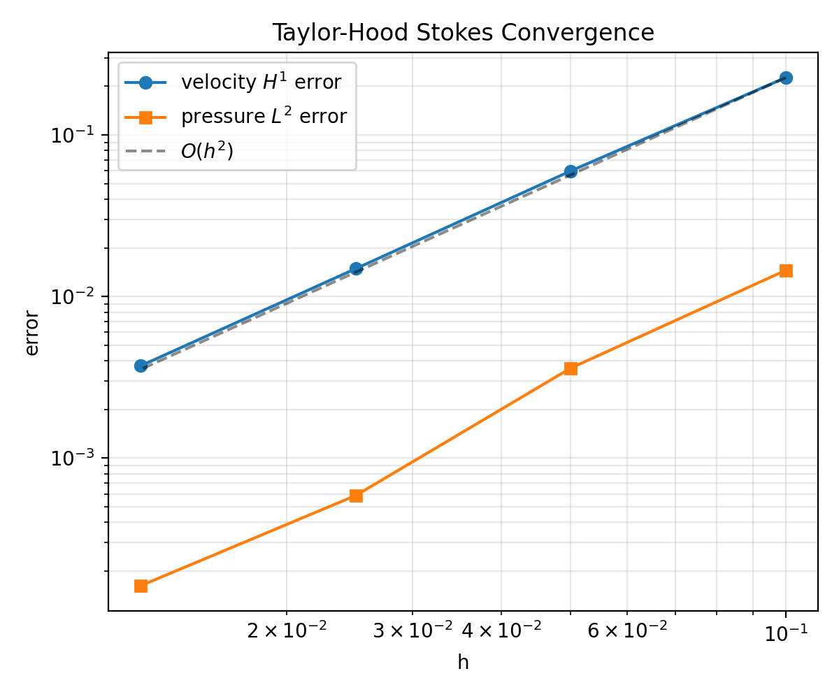
Fig. 59 Velocity \(H^1\) and pressure \(L^2\) errors under uniform h-refinement, both tracking the \(O(h^2)\) reference slope.

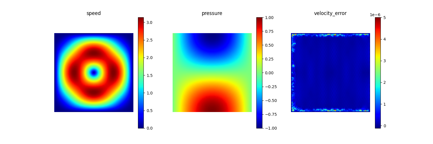
Fig. 60 Finest-level solution: speed magnitude, P1 pressure (prolonged to the P2 mesh points for plotting), and the pointwise velocity error against the exact solution.

Running it

cd examples/fluid/stokes_taylor_hood
python stokes_taylor_hood.py   # convergence table + two PNGs

The four-level study runs in a few minutes on CPU; the finest level has ~67k DOFs.

What’s next

• Lid-Driven Cavity — add convection and Picard linearization to this exact assembler.

• Mixed Assembly — the full mixed-assembly contract (fields, layout, load vectors, generalized order pairs).

• Sparse Solvers — solver backends for the saddle-point system.