Modal Analysis

Two examples that solve generalized eigenproblems instead of driven systems — one photonic, one structural. Both follow the same recipe: assemble two (or three) matrices with the builtin assemblers, hand them to a shift-invert sparse eigensolver, and read physical frequencies / propagation constants off the spectrum:

mesh -> assemble (K, M, ...) -> shift-invert eigsh -> modes + frequencies

Each validates against a closed-form reference (Marcatili’s slab approximation, Euler-Bernoulli beam theory).

Rectangular waveguide modes (photonics)

examples/wave/wave_guide_mode/waveguide_modes.py computes the guided modes of a rectangular dielectric waveguide from its 2D cross-section. In the weakly-guiding scalar approximation the transverse field \(E(x,y)\) and propagation constant \(\beta\) satisfy

\[\big(K - k_0^2 M_\varepsilon\big)\,E \;=\; -\beta^2\, M\,E,\]

built from three builtins — stiffness (LaplaceElementAssembler), mass (MassElementAssembler), and the index-weighted mass \(M_\varepsilon = \int n^2\,\phi_i\phi_j\) (ScaledMassElementAssembler). A mode is guided when its effective index \(n_{\text{eff}} = \beta/k_0\) falls between the cladding and core indices; the default geometry (\(18 \times 14\) µm core, \(n = 1.450/1.444\), \(\lambda_0 = 1.55\) µm) carries seven guided modes, and the computed effective indices agree with Marcatili’s separable slab approximation to \(\sim 10^{-4}\).

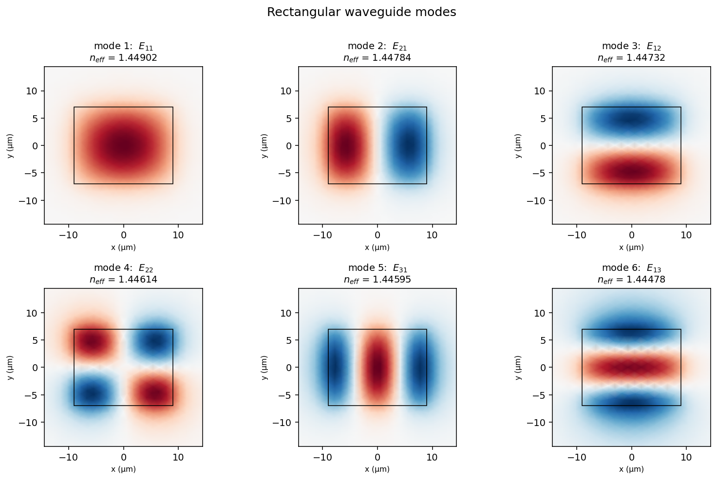
Fig. 50 The guided transverse fields \(E_{pq}\) (red/blue = field sign, core outlined), labelled by their lobe counts along \(x\) and \(y\) — the fundamental \(E_{11}\), the dipole pair \(E_{21}/E_{12}\), and the higher-order modes.

Cantilever beam vibration (structural)

examples/solid/beam_vibration_analysis/vibration_cylinder.py runs the classic free-vibration analysis of a clamped-free steel cylinder (\(L = 1\) m, \(R = 25\) mm) in 3D linear elasticity:

\[K\,\phi = \omega^2 M\,\phi,\]

with \(K\) from LinearElasticityElementAssembler and the consistent vector mass built from the scalar mass matrix (\(M_{\text{vec}} = \rho\, M_{\text{scalar}} \otimes I_3\)). The clamped base is removed by the usual Condenser mask. On top of the modes, a modal FRF — the tip response to a transverse tip force with 1% modal damping — shows the resonance/antiresonance structure.

The first bending frequency comes out at 37.2 Hz vs Euler-Bernoulli theory’s 36.2 Hz (+3% with P1 tets, converging with refinement); because the section is circular, every bending mode arrives as a near-degenerate pair (two orthogonal bending planes), followed by the first torsion and axial modes.

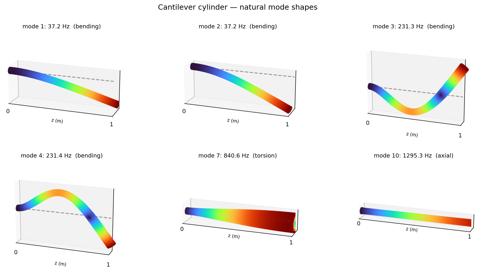
Fig. 51 Deformed mode shapes (displacement magnitude, exaggerated): the bending pairs, first torsion, and first axial mode.

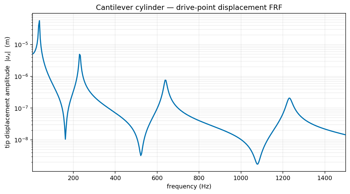
Fig. 52 Dynamic amplification \(|u_x|/u_{\text{static}}\) at the tip — flat at 1 below the first resonance, peaking on each bending mode, dropping into antiresonances between them.

Running them

cd examples/wave/wave_guide_mode && python waveguide_modes.py
cd examples/solid/beam_vibration_analysis && python vibration_cylinder.py

Both expose run_demo(...) plus geometry / mode-count / mesh-size flags (--help lists them). The eigensolves run through SciPy’s shift-invert Lanczos on the assembled sparse matrices — post-processing only, the assembly core stays torch.

What’s next

• Phononic Crystals (Bloch-Floquet) — eigenproblems with Bloch-Floquet phase boundary conditions (band structures).

• Open-Domain Wave (PML & Ports) — the driven counterparts: ports and PML.

• Solid Mechanics — the static and nonlinear solid-mechanics ladder.