Plasticity with Newton’s Method
The elastic-plastic thick-walled cylinder [Hill1950]: a long tube under
internal pressure, loaded until the whole wall flows. The script
examples/solid/plasticity_cylinder/plasticity_cylinder.py solves it in
plane strain with von Mises (J2) plasticity and checks the result against the
closed-form elastic response and the limit pressure.
The new ingredient over Plasticity (J2 with Isotropic Hardening) is the consistent tangent.
There, every load step minimizes an incremental energy with L-BFGS. Here,
every load step is solved by Newton’s method with the derivative of the
stress update itself, so the iterations converge quadratically: three to five
per plastic load step. The plastic state stays at the quadrature points and
reaches the assemblers as quadrature_data.
Model
Small strains, \(\boldsymbol{\varepsilon} = \boldsymbol{\varepsilon}^e + \boldsymbol{\varepsilon}^p\), isotropic elasticity with shear modulus \(\mu\) and bulk modulus \(\kappa\), the von Mises yield function with linear isotropic hardening,
(\(\mathbf{s}\) the stress deviator, \(p\) the equivalent plastic strain, \(H = 0\) perfect plasticity) and associated flow. Plane strain keeps \(\varepsilon_{zz} = 0\), so the strain and stress are carried as \(3 \times 3\) tensors: \(\sigma_{zz}\) is not zero, and neither is \(\varepsilon^p_{zz}\).
Radial return. In a load step the total strain \(\boldsymbol{\varepsilon}\) at a quadrature point is given, and the state at the start of the step is \((\boldsymbol{\varepsilon}^p_n, p_n)\). The trial stress \(\boldsymbol{\sigma}^{tr} = \mathbb{C} : (\boldsymbol{\varepsilon} - \boldsymbol{\varepsilon}^p_n)\) has the deviator \(\mathbf{s}^{tr}\) and the von Mises stress \(q^{tr}\). If \(f^{tr} = q^{tr} - (\sigma_y + H p_n) \le 0\) the step is elastic. Otherwise the deviator is scaled back onto the yield surface:
Consistent tangent [Simo1985] [deSouzaNeto2008]. Differentiating this update, not the continuum relation, gives the moduli Newton needs:
on plastic points, and the elastic moduli elsewhere. radial_return
computes the stress, the new state and these moduli for all quadrature points
at once:
def radial_return(eps, eps_p, p, mat: J2Material):
    """Stress update of J2 plasticity at every quadrature point.

    Parameters
    ----------
    eps : torch.Tensor
        Total strain ``[..., 3, 3]`` at the end of the step (plane strain:
        the third row and column are zero).
    eps_p, p : torch.Tensor
        Plastic strain ``[..., 3, 3]`` and equivalent plastic strain ``[...]``
        at the start of the step.

    Returns
    -------
    sigma : torch.Tensor
        Stress ``[..., 3, 3]``.
    eps_p, p : torch.Tensor
        Updated plastic state.
    C : torch.Tensor
        Consistent tangent d sigma / d eps ``[..., 3, 3, 3, 3]``:
        kappa 1x1 + 2 mu (1 - 3 mu dp / q) I_dev + 6 mu^2 (dp / q - 1 / (3 mu + H)) N x N
        on plastic points, kappa 1x1 + 2 mu I_dev on elastic ones, with q the
        trial von Mises stress and N the unit trial deviator
        (de Souza Neto, Peric and Owen, 2008, box 7.4).
    """
    mu, kappa, H = mat.mu, mat.kappa, mat.H
    one = torch.eye(3, dtype=eps.dtype, device=eps.device)
    ee = eps - eps_p                                                # trial elastic strain
    tr = ee.diagonal(dim1=-2, dim2=-1).sum(-1)
    s = 2 * mu * (ee - tr[..., None, None] / 3 * one)              # trial deviatoric stress
    norm_s = torch.sqrt((s * s).sum((-2, -1)))
    q = math.sqrt(1.5) * norm_s                                     # trial von Mises stress
    f = q - (mat.sigma_y + H * p)
    plastic = f > 0
    dp = torch.where(plastic, f, torch.zeros_like(f)) / (3 * mu + H)
    N = s / torch.where(plastic, norm_s, torch.ones_like(norm_s))[..., None, None]
    flow = math.sqrt(1.5) * dp[..., None, None] * N                 # plastic strain increment
    sigma = kappa * tr[..., None, None] * one + s - 2 * mu * flow

    q_safe = torch.where(plastic, q, torch.ones_like(q))
    a = torch.where(plastic, 3 * mu * dp / q_safe, torch.zeros_like(q))
    b = torch.where(plastic, 6 * mu**2 * (dp / q_safe - 1 / (3 * mu + H)), torch.zeros_like(q))
    ones = torch.einsum("ij,kl->ijkl", one, one)
    sym = 0.5 * (torch.einsum("ik,jl->ijkl", one, one) + torch.einsum("il,jk->ijkl", one, one))
    C = (kappa * ones + (2 * mu * (1 - a))[..., None, None, None, None] * (sym - ones / 3)
         + b[..., None, None, None, None] * torch.einsum("...ij,...kl->...ijkl", N, N))
    return sigma, eps_p + flow, p + dp, C
The test suite compares the tangent with a forward-mode autodiff derivative
of the stress update, torch.func.jvp. That derivative is also the way to
get the tangent of a model without a closed form.
Quadrature-point data
The stress and the moduli are arrays over the quadrature points,
[n_elements, n_quadrature, ...]. Passed as quadrature_data, an entry
reaches forward as its value at the current point, under its own name:
class InternalForce(NodeAssembler):
    """f_i = int sigma . grad N_i dx, sigma given at the quadrature points."""

    def forward(self, gradv, sigma):
        return sigma @ gradv
class Tangent(ElementAssembler):
    """K_ij = int grad N_i . C . grad N_j dx, C given at the quadrature points."""

    def forward(self, gradu, gradv, C):
        return torch.einsum("j,ajbl,l->ab", gradu, C, gradv)
The internal-force vector is InternalForce(quadrature_data={"sigma": sigma})
and the stiffness matrix Tangent(quadrature_data={"C": C}), with the
in-plane parts of the \(3 \times 3\) tensors. The pressure acts along the
outward unit normal of the inner wall, which forward of a
FacetAssembler receives as n:
class Pressure(FacetAssembler):
    """Nodal forces of a unit pressure, f_i = -int N_i n ds (n: outward normal)."""

    def forward(self, v, n):
        return -v[:, None] * n
Newton’s method
Each load step iterates until the residual on the free degrees of freedom is
below \(10^{-10}\) of the applied or reaction forces. The first iteration
starts from the converged state of the previous step and carries the change of
the prescribed displacements through the whole body (a linear predictor,
through update_dirichlet()); the later iterations
keep the prescribed values. The plastic state is committed once the step has
converged, so every iteration returns from the same state.
    def solve_step(self, f_ext, prescribed=None):
        """Equilibrium for the external forces ``f_ext`` [n_points * 2] and the
        values ``prescribed`` on the fixed dofs (default: keep them).

        The first Newton iteration starts from the converged state and carries
        the change of the prescribed values into the whole body (the linear
        predictor); the later ones keep them. Returns the relative residual
        after every Newton update.
        """
        jump = torch.zeros_like(self.u)
        if prescribed is not None:
            jump = torch.where(self.fixed, prescribed - self.u, jump)
        history = []
        for it in range(self.max_iterations + 1):
            R, (sigma, eps_p, p, C) = self.residual(self.u, f_ext)
            if it > 0:
                scale = max(float(torch.linalg.vector_norm(f_ext)), float(torch.linalg.vector_norm(R[self.fixed])),
                            1e-300)
                history.append(float(torch.linalg.vector_norm(R[~self.fixed])) / scale)
                if history[-1] <= self.tol:
                    break
            if it == self.max_iterations:
                raise RuntimeError(f"Newton did not converge: relative residuals {history}")
            K = self.tangent(quadrature_data={"C": C[..., :2, :2, :2, :2]})
            self.condenser.update_dirichlet(jump if it == 0 else torch.zeros_like(jump))
            K_free, rhs = self.condenser(K, -R)
            du = K_free.solve(rhs, backend=self.linear_solver).to(rhs.device)   # SciPy answers on the host
            self.u = self.u + self.condenser.recover(du)
        self.eps_p, self.p, self.sigma = eps_p, p, sigma   # commit the converged state
        self.reaction = R
        return history
The thick-walled cylinder
Geometry: a quarter of the tube, \(a = 100\) mm, \(b = 200\) mm, plane strain, with \(u_y = 0\) on the \(x\) axis and \(u_x = 0\) on the \(y\) axis.
Material: \(E = 200\) GPa, \(\nu = 0.3\), \(\sigma_y = 250\) MPa, perfect plasticity.
Loading: the inner wall is pushed out to six times the first-yield displacement in 30 steps. Under this displacement control the pressure is the reaction on the inner wall, projected on the nodal forces of a unit pressure.
--control pressureraises the pressure instead, which stops short of the limit.Mesh: six-node triangles on a polar grid, built with NumPy. The radial spacing grows with \(r\) and the mid-edge nodes of the arcs lie on the circles (825 nodes).
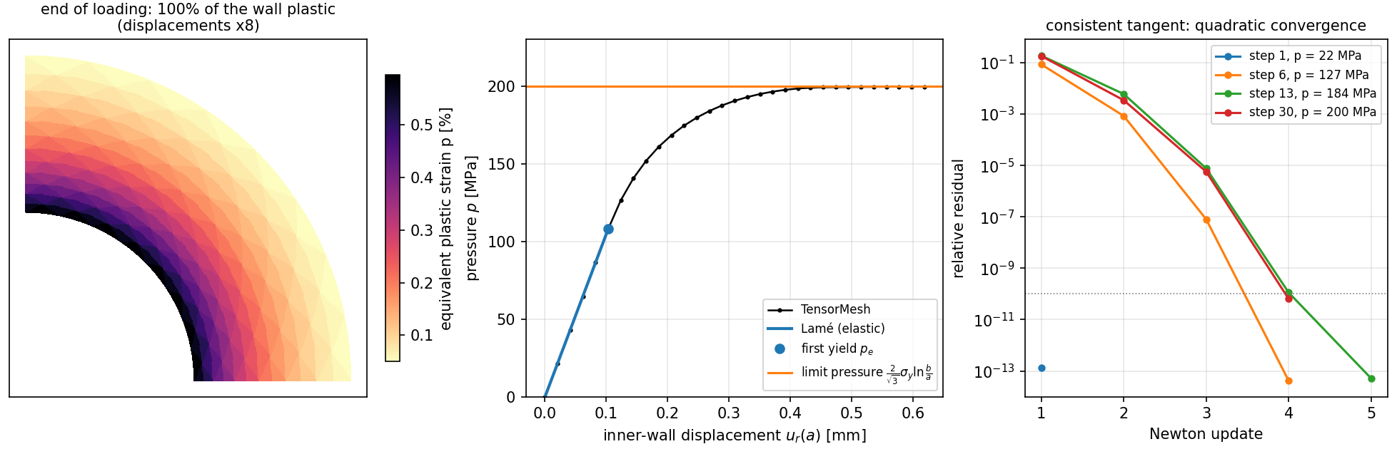
Fig. 62 Output of plasticity_cylinder.py. Left: the equivalent plastic strain
at the end of loading. Middle: the pressure against the inner-wall
displacement, with the Lamé line, the first-yield point and the limit
pressure. Right: the Newton residuals of an elastic step, the first
plastic step, a half-plastic step and the last one.
The response follows the Lamé line until the inner wall yields at \(p_e = 108.1\) MPa. The plastic zone then spreads outward, and the pressure rises more and more slowly. Once the zone reaches the outer wall the tube flows at a nearly constant pressure: the last step carries 199.7 MPa, within 0.2 % of the limit pressure \(\tfrac{2}{\sqrt3}\, \sigma_y \ln(b/a) = 200.1\) MPa, approached from below. Elastic steps take one Newton update and plastic steps three to five, with the residual roughly squared from one to the next.
Verification
tests/assemble/test_plasticity_cylinder_example.py checks:
Return map: plastic points end on the yield surface, elastic points keep the elastic stress, the plastic flow is deviatoric, and the tangent equals a forward-mode autodiff derivative of the stress update.
Stiffness matrix: the assembled tangent against central differences of the residual.
Elastic range: the inner-wall displacement against the Lamé solution,
\[\frac{p}{u_r(a)} = \frac{E\, (b^2 - a^2)}{(1 + \nu)\, a\, \bigl[(1 - 2\nu)\, a^2 + b^2\bigr]},\]under pressure and displacement control.
First yield: no plastic point below the first-yield displacement, and only in the innermost elements just above it.
Collapse: the pressure of a perfectly plastic tube rises to the limit pressure within 1 %, from below, and Newton converges in at most six updates per load step.
Devices: CUDA against CPU, when a GPU is present.
Running it
cd examples/solid/plasticity_cylinder
python plasticity_cylinder.py                       # displacement control
python plasticity_cylinder.py --control pressure    # up to 0.98 of the limit pressure
python plasticity_cylinder.py --hardening 2000      # H = 2 GPa
The default run takes a few seconds on a CPU. --device cuda assembles on
the GPU; the Newton systems then use cuDSS if torch-sla has it, and SciPy on
the host otherwise.
Notes
Why displacement control. Under pressure control a perfectly plastic tube cannot be loaded past the limit pressure, and close to it the tangent becomes singular. Prescribing the inner-wall displacement follows the plateau.
Elements. Plastic flow preserves volume, and linear (constant-strain) triangles lock under this constraint in plane strain, overestimating the collapse load [Nagtegaal1974]. The quadratic triangles used here reach the limit pressure within 0.2 %.
The first iteration. Moving only the boundary nodes to their new prescribed positions before the first solve strains only the layer of elements next to them, and can make it yield spuriously. The linear predictor spreads the change through the body first.
What’s next
Plasticity (J2 with Isotropic Hardening): the same J2 model as an incremental energy, minimized with L-BFGS, with
J2Plasticity.Forms:
quadrature_data,nand the other namesforwardcan take.
R. Hill, The Mathematical Theory of Plasticity, Oxford University Press, 1950.
J. C. Simo and R. L. Taylor, Consistent tangent operators for rate-independent elastoplasticity, Computer Methods in Applied Mechanics and Engineering, 48(1):101–118, 1985.
E. A. de Souza Neto, D. Perić and D. R. J. Owen, Computational Methods for Plasticity: Theory and Applications, Wiley, 2008.
J. C. Nagtegaal, D. M. Parks and J. R. Rice, On numerically accurate finite element solutions in the fully plastic range, Computer Methods in Applied Mechanics and Engineering, 4(2):153–177, 1974.