Helmholtz Scattering (DtN Boundary Treatment)¶

The two self-contained scripts in examples/wave/helmholtz_dtn treat full-space scattering and scattering by a horizontally periodic layer. The same scalar formulation applies to electromagnetic TE/TM polarizations and to acoustic pressure waves.

For absorbing layers and port boundaries instead of exact DtN maps, see Open-Domain Wave (PML & Ports).

We use the time convention \(e^{-i\omega t}\) and write

\[\nabla\!\cdot\!\bigl(a(x)\nabla u\bigr)+\omega^2b(x)u=0.\]

Here \(a,b\in L^\infty\) are real-valued, uniformly positive scalar functions. Both coefficients may vary in space; the piecewise-constant materials used by the analytical examples below are a special case.

Table 1 Physical meaning of the scalar coefficients¶
Model	Scalar field	\(a(x)\)	\(b(x)\)
`TM_EZ`	\(u=E_z\)	\(\mu(x)^{-1}\)	\(\varepsilon(x)\)
`TE_HZ`	\(u=H_z\)	\(\varepsilon(x)^{-1}\)	\(\mu(x)\)
Acoustic pressure	\(u=p\)	\(\rho(x)^{-1}\)	\(K(x)^{-1}=1/[\rho(x)c(x)^2]\)

The electromagnetic rows use the project convention that TM_EZ names the out-of-plane electric field and TE_HZ the out-of-plane magnetic field. The demos use normalized units. With relative material parameters, their coefficient pairs are \((a,b)=(\mu_r^{-1},\varepsilon_r)\) for TM_EZ and \((a,b)=(\varepsilon_r^{-1},\mu_r)\) for TE_HZ. In any homogeneous region \(j\), the corresponding wavenumber is

\[k_j=\omega\sqrt{b_j/a_j}.\]

Run the examples

python examples/wave/helmholtz_dtn/circular_dtn.py
python examples/wave/helmholtz_dtn/periodic_dtn.py

Full-space scattering¶

General scattering problem¶

Let \(D\Subset\mathbb R^2\) be a bounded obstacle or penetrable inclusion with boundary \(\Gamma\). Outside a bounded region the material is homogeneous, with constants \(a_0,b_0>0\) and exterior wavenumber \(k_0=\omega\sqrt{b_0/a_0}\).

Before choosing a particular incident wave, let \(u^{\rm inc}\) be any entire solution of the exterior equation

\[\Delta u^{\rm inc}+k_0^2u^{\rm inc}=0.\]

The scatterer generates an outgoing field \(u^{\rm sc}\). In the exterior, the total field is

\[u=u^{\rm inc}+u^{\rm sc}.\]

The coefficients themselves are not compactly supported: waves must propagate through the exterior medium. It is the material contrast that is compactly supported,

\[\operatorname{supp}(a-a_0)\cup\operatorname{supp}(b-b_0) \Subset\mathbb R^2.\]

For an obstacle, the unknown total field is defined in the exterior of \(D\). For a penetrable inclusion, it is defined across the whole plane; the coefficients may vary inside the compact contrast region. The circular verification case later specializes the inclusion to constants \((a_1,b_1)\).

Physical boundary and interface conditions¶

The three cases differ only at the physical circle. With \(\nu\) pointing from \(D\) into the exterior, they impose

\[\begin{split}\begin{aligned} u&=0 &&\text{on }\Gamma &&\text{(Dirichlet obstacle)},\\ a_0\partial_\nu u&=0 &&\text{on }\Gamma &&\text{(Neumann obstacle)},\\ [u]&=0,\qquad [a\partial_\nu u]=0 &&\text{on }\Gamma &&\text{(penetrable inclusion)}. \end{aligned}\end{split}\]

For the transmission case the jump is the interior trace minus the exterior trace. Thus both the field and the weighted normal flux are continuous.

Full-space radiation condition¶

The scattered field is outgoing. For the \(e^{-i\omega t}\) convention it satisfies the two-dimensional Sommerfeld condition

\[\lim_{r\to\infty}\sqrt r\, \left(\partial_ru^{\rm sc}-ik_0u^{\rm sc}\right)=0\]

uniformly in direction. This condition selects Hankel functions of the first kind and, under the stated positive-material assumptions, singles out the outgoing solution.

Circular DtN truncation¶

Choose an artificial circle \(\Gamma_R=\{r=R\}\) enclosing the physical scatterer and every material contrast. If

\[\widehat\phi_m=\frac{1}{2\pi}\int_0^{2\pi} \phi(\theta)e^{-im\theta}\,d\theta,\]

then the exact exterior Fourier–Hankel DtN map is

\[T_R\phi =\sum_{m\in\mathbb Z}\tau_m\widehat\phi_m e^{im\theta}, \qquad \tau_m=k_0\frac{H_m^{(1)\prime}(k_0R)}{H_m^{(1)}(k_0R)}.\]

Because \(\partial_n-T_R\) annihilates every outgoing Hankel mode, the unbounded radiation condition is equivalent to the total-field boundary condition

\[\partial_nu-T_Ru=g_R, \qquad g_R=\partial_nu^{\rm inc}-T_Ru^{\rm inc} \quad\text{on }\Gamma_R,\]

where \(n=e_r\) is the outward normal of the truncated domain.

Full-space weak form¶

Let \(\Omega_R=B_R\setminus\overline D\) for an obstacle and \(\Omega_R=B_R\) for transmission. The trial and test space is

\[V_D=\{v\in H^1(\Omega_R):v|_\Gamma=0\}\]

for the Dirichlet obstacle, and \(V=H^1(\Omega_R)\) for the Neumann and transmission cases. Find \(u\) in the appropriate affine trial space such that, for every test function \(v\) in its homogeneous counterpart,

\[\int_{\Omega_R}a\nabla u\cdot\nabla\overline v -\omega^2\int_{\Omega_R}bu\overline v -a_0\langle T_Ru,v\rangle_{\Gamma_R} =a_0\langle g_R,v\rangle_{\Gamma_R}.\]

The Dirichlet trace is imposed strongly with Condenser. The homogeneous Neumann condition is natural, so it contributes no boundary integral. For transmission, a conforming mesh and element-wise \(a,b\) enforce \([u]=[a\partial_\nu u]=0\) through the weak form.

Periodic scattering¶

Periodic material and vertical compactness¶

Let \(x_1\) be periodic with period \(L\). The coefficients satisfy

\[a(x_1+L,x_2)=a(x_1,x_2), \qquad b(x_1+L,x_2)=b(x_1,x_2).\]

A nontrivial periodic coefficient cannot be compactly supported in the full plane. The correct open-domain assumption is compactness in the vertical direction within one periodic cell: the coefficients become constant above and below a bounded strip. In the present demos,

\[\exists\,y_-<y_+:\qquad a(x_1,x_2)=a_0,\quad b(x_1,x_2)=b_0 \quad\text{for }x_2\notin[y_-,y_+],\ 0<x_1<L.\]

The slab has material \((a_1,b_1)\) in \(0<x_2<h\) and material \((a_0,b_0)\) in both exterior half-spaces. The wall problems retain only \(x_2>0\): the same finite layer is backed by a physical boundary at \(x_2=0\) and is open above.

Bloch condition¶

For a prescribed horizontal Bloch wavenumber \(\alpha\), the total field satisfies

\[u(L,x_2)=e^{i\alpha L}u(0,x_2), \qquad \partial_{x_1}u(L,x_2) =e^{i\alpha L}\partial_{x_1}u(0,x_2).\]

Since \(a\) is periodic, the horizontal material flux carries the same phase. Trial and test functions use this quasi-periodicity; consequently \(\overline v\) carries the conjugate phase and the two lateral weak-form boundary terms cancel.

General incident, scattered, and total fields¶

A downward plane wave enters from the top reference line \(\Gamma_+=\{x_2=y_t\}\):

\[u^{\rm inc} =Ae^{i\alpha x_1-i\beta_{0,0}(x_2-y_t)}.\]

For \(m\in\mathbb Z\), define

\[\alpha_m=\alpha+\frac{2\pi m}{L}, \qquad \beta_{j,m}=\sqrt{k_j^2-\alpha_m^2}.\]

The incident order is assumed to propagate, \(|\alpha|<k_0\), so that \(\beta_{0,0}>0\) and its incoming power is nonzero. For every retained order, the outgoing branch has \(\beta_{j,m}>0\) for a propagating mode and \(\operatorname{Im}\beta_{j,m}>0\) for an evanescent mode; a grazing mode has \(\beta_{j,m}=0\). The demo parameters avoid Wood anomalies, where a retained \(\alpha_m^2=k_j^2\); such cutoffs require separate treatment in the Rayleigh expansion and power normalization. The scattered field above the structure has the outgoing Rayleigh expansion

\[u^{\rm sc} =\sum_{m\in\mathbb Z}r_m e^{i\alpha_mx_1+i\beta_{t,m}(x_2-y_t)}, \qquad x_2\geq y_t.\]

Thus the total field at the top is

\[u=u^{\rm inc}+u^{\rm sc}.\]

For a two-port slab there is no incident wave from below, so the lower total field is the transmitted outgoing field

\[u=u^{\rm tr} =\sum_{m\in\mathbb Z}t_m e^{i\alpha_mx_1-i\beta_{b,m}(x_2-y_b)}, \qquad x_2\leq y_b.\]

These Rayleigh expansions are the periodic counterparts of the Sommerfeld radiation condition.

Physical interfaces and wall conditions¶

The three configurations are:

slab: field and weighted flux are continuous at both flat material interfaces, \([u]=0\) and \([a\partial_\nu u]=0\) at \(x_2=0,h\), with open ports above and below;
dirichlet: the layer interface at \(x_2=h\) satisfies the same two transmission conditions and \(u=0\) at the wall \(x_2=0\);
neumann: the interface conditions hold at \(x_2=h\) and \(a\partial_\nu u=0\) at \(x_2=0\).

Rayleigh DtN truncation¶

Let \(\Gamma_-\) denote the bottom reference line of the slab. With modal coefficients taken in the quasi-periodic basis \(e^{i\alpha_mx_1}\), define

\[T_\pm\phi =\sum_{m\in\mathbb Z}i\beta_{\pm,m}\widehat\phi_m e^{i\alpha_mx_1}.\]

Both symbols are \(i\beta_{\pm,m}\) because each operator uses the outward normal of the truncated cell: \(n=+e_2\) at the top and \(n=-e_2\) at the bottom. The top total-field condition is

\[\partial_nu-T_+u=g_+, \qquad g_+=-2i\beta_{0,0}Ae^{i\alpha x_1} \quad\text{on }\Gamma_+.\]

For the slab, the lower field is purely outgoing, hence

\[\partial_nu-T_-u=0 \quad\text{on }\Gamma_-.\]

Periodic weak form¶

Let \(\Omega_L\) be one truncated period cell and define

\[V_\alpha=\left\{v\in H^1(\Omega_L): v(L,x_2)=e^{i\alpha L}v(0,x_2)\right\}.\]

For the Dirichlet wall use \(V_{\alpha,D}=\{v\in V_\alpha:v=0\text{ on }x_2=0\}\); the slab and Neumann wall use \(V_\alpha\). With \(\delta_{\rm slab}=1\) for the slab and zero for a wall, find \(u\) in the corresponding trial space such that

\[\int_{\Omega_L}a\nabla u\cdot\nabla\overline v -\omega^2\int_{\Omega_L}bu\overline v -a_t\langle T_+u,v\rangle_{\Gamma_+} -\delta_{\rm slab}a_b\langle T_-u,v\rangle_{\Gamma_-} =a_t\langle g_+,v\rangle_{\Gamma_+}\]

for every homogeneous test function \(v\). In the present slab \(a_t=a_b=a_0\). A Neumann wall is natural and contributes no lower boundary term. This form fixes the implementation order: assemble the volume and DtN operators, apply BlochReducer to form \(T^HAT\) and \(T^Hb\), then apply Condenser only for the Dirichlet wall.

Layered exact solutions for verification¶

The general periodic problem may couple many Rayleigh orders. For code verification, the flat interfaces preserve the incident order. With \(\beta=\beta_{0,0}\) and \(\gamma=\beta_{1,0}\), the incident, scattered, and top total fields are

\[\begin{split}\begin{aligned} u^{\rm inc}&=Ae^{i\alpha x_1-i\beta(x_2-y_t)},\\ u^{\rm sc}&=re^{i\alpha x_1+i\beta(x_2-y_t)},\\ u_{\rm top}&=u^{\rm inc}+u^{\rm sc}. \end{aligned}\end{split}\]

The layer and lower transmitted total fields are

\[\begin{split}\begin{aligned} u_{\rm layer}&=e^{i\alpha x_1} \left[pe^{-i\gamma x_2}+qe^{i\gamma x_2}\right],\\ u_{\rm bottom}&=u^{\rm tr} =te^{i\alpha x_1-i\beta(x_2-y_b)}. \end{aligned}\end{split}\]

Continuity of \(u\) and \(a\partial_{x_2}u\) at \(x_2=h\) and \(x_2=0\) gives the four-by-four system for \((r,p,q,t)\) used in the script. A wall removes the lower port and uses the layer total fields

\[u_D=d\,e^{i\alpha x_1}\sin(\gamma x_2), \qquad u_N=d\,e^{i\alpha x_1}\cos(\gamma x_2).\]

The sine enforces the Dirichlet trace and the cosine has zero normal derivative at \(x_2=0\); matching at \(h\) gives a two-by-two system for \((r,d)\).

The periodic solve uses TensorMesh’s public constraint operators: reduce() forms \(T^H A T\), reduce_rhs() forms \(T^H b\), and reduce_mask() maps the wall DOFs onto the reduced DOFs for the Condenser:

Listing 14 examples/wave/helmholtz_dtn/periodic_dtn.py (constraint essence)¶

reducer = BlochReducer(mesh.points, [[period, 0.0]], sign=+1)
wavevector = torch.tensor([alpha, 0.0], dtype=torch.float64)
reduced_matrix = reducer.reduce(matrix, wavevector)       # T^H A T
reduced_rhs = reducer.reduce_rhs(rhs, wavevector)         # T^H b

if case == "dirichlet":
    master_mask = reducer.reduce_mask(bottom_mask)
    zero_trace = torch.zeros(int(master_mask.sum()), dtype=torch.complex128)
    condenser = Condenser(master_mask, dirichlet_value=zero_trace)
    inner_matrix, inner_rhs = condenser(reduced_matrix, reduced_rhs)
    inner_solution = inner_matrix.solve(inner_rhs, backend="scipy", method="lu")
    reduced_solution = condenser.recover(inner_solution)
else:                                                     # natural Neumann wall
    reduced_solution = reduced_matrix.solve(
        reduced_rhs, backend="scipy", method="lu"
    )

solution = reducer.recover(reduced_solution, wavevector)

Numerical, exact, and error fields for the two-port periodic slab. — Fig. 56 Two-port slab.¶

Numerical, exact, and error fields for the Dirichlet-backed layer. — Fig. 57 Dirichlet-backed layer.¶

Numerical, exact, and error fields for the Neumann-backed layer. — Fig. 58 Neumann-backed layer.¶

Lower-case \(r_m,t_m\) denote complex amplitudes. Reflectance and transmittance are power fractions:

\[\mathcal R_m= \frac{\operatorname{Re}(a_t\beta_{t,m})} {\operatorname{Re}(a_t\beta_{t,0})} \left|\frac{r_m}{A}\right|^2, \qquad \mathcal T_m= \frac{\operatorname{Re}(a_b\beta_{b,m})} {\operatorname{Re}(a_t\beta_{t,0})} \left|\frac{t_m}{A}\right|^2.\]

A wall has no lower radiation port, so the script reports only \(r\) and \(\mathcal R\); it does not invent zero transmission values.

TensorMesh assembly details

The reading order mirrors the official Helmholtz demo:

keep mesh geometry, basis functions, Jacobians, and quadrature in float64;
promote HelmholtzAssembler to complex128 and assemble \(a\nabla u\cdot\nabla v-\omega^2buv\) with ElementAssembler;
compute modal traces with FacetAssembler;
add the nonlocal DtN block to the TensorMesh sparse COO matrix;
impose constraints, solve the general complex system, and compare with the exact field.

The weighted volume form is the only problem-specific element assembler. All basis evaluation, quadrature, Jacobian transformations, element indexing, and global sparse scatter remain inside TensorMesh:

Listing 15 Weighted complex Helmholtz assembly (shared pattern)¶

class HelmholtzAssembler(ElementAssembler):
    def forward(self, gradu, gradv, u, v, a, b, omega_sq):
        return a * (gradu @ gradv) - omega_sq * b * u * v

assembler = HelmholtzAssembler.from_mesh(mesh, quadrature_order=4)
assembler.type(torch.complex128)
volume = assembler(
    points=mesh.points,
    element_data={
        "a": a.to(torch.complex128),
        "b": b.to(torch.complex128),
        "omega_sq": torch.full_like(a, omega**2, dtype=torch.complex128),
    },
)

TensorMesh 0.2.0 also provides FacetBilinearAssembler for local Robin or impedance matrices. A DtN map is nonlocal, however, so these demos intentionally use FacetAssembler for modal moments and form the low-rank boundary block only after integration.

The facet path is real, so each exponential is integrated as cosine and negative-sine channels, then combined as complex128. If \(\Psi\) is the modal moment matrix, both demos use

Psi.conj() @ torch.diag(symbols) @ Psi.T

The last factor is a plain transpose because \(\Psi^Tu\) gives modal coefficients. The matrix is not assumed Hermitian or positive definite. The scripts call TensorMesh SparseMatrix.solve with the SciPy LU backend selected explicitly instead of requesting an SPD solver.

For a periodic Dirichlet wall, the operation order is essential:

assemble the full volume and DtN matrix;
form \(T^HAT\) and \(T^Hb\) with BlochReducer(sign=+1);
map the complete bottom trace to unique Bloch master degrees of freedom;
apply Condenser and solve;
recover through Condenser and then BlochReducer.

The Neumann wall is a natural weak boundary and skips condensation. The tests compare the Bloch reductions with an explicit matrix \(T\), substitute orders \(-2,0,3\) into the circular boundary conditions, check P1 convergence, and verify amplitudes, powers, Bloch traces, and nonzero-mode leakage.

Plots and analytical verification

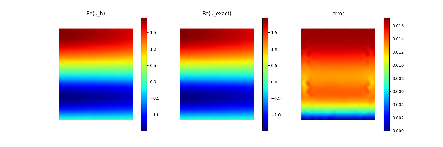
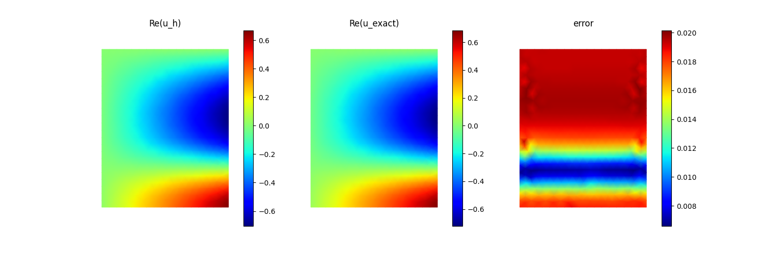
Both scripts use plot() rather than constructing an independent plotting pipeline:

Listing 16 Numerical field, exact field, and pointwise error¶

numerical = solution.detach().cpu()
reference = torch.as_tensor(exact, dtype=torch.complex128)
fields = {
    "Re(u_h)": numerical.real,
    "Re(u_exact)": reference.real,
    "error": abs(numerical - reference),
}
mesh.plot(fields, save_path=filename, show_mesh=False)

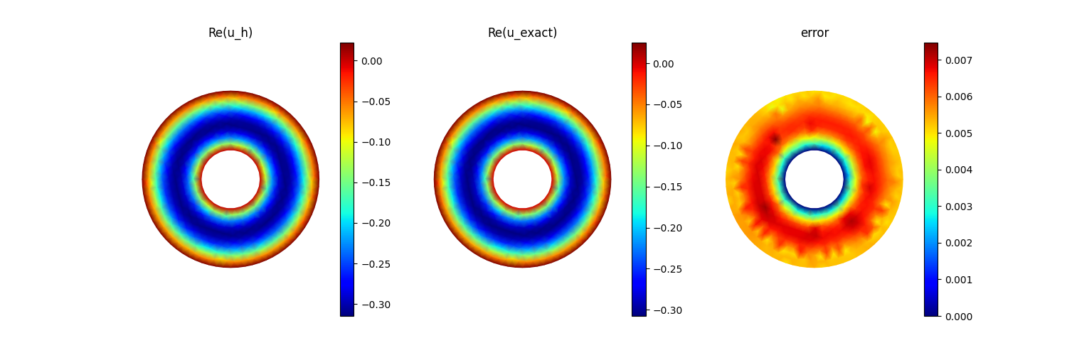
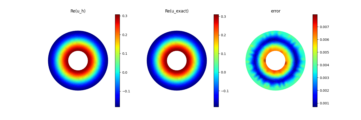
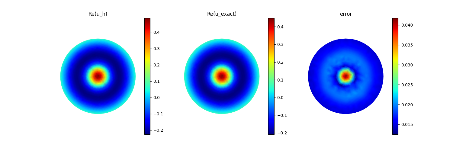
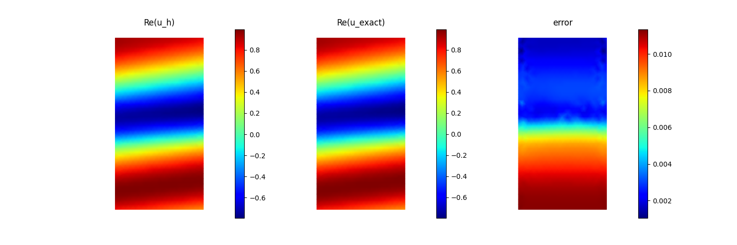
With the default CPU complex128 settings, the three circular cases have relative nodal errors below \(5.6\times10^{-2}\) and fitted P1 convergence orders between \(1.71\) and \(1.74\). For the periodic cases, the relative errors in the analytical amplitudes remain below \(2.0\times10^{-2}\), the energy-balance residual is below \(2.0\times10^{-15}\), and the recovered Bloch trace agrees to machine precision. The committed figures show the numerical field, analytical field, and their pointwise error for every case.