Phononic Crystals (Bloch-Floquet)
Two-dimensional acoustic phononic-crystal examples in
examples/wave/phononic_crystal_2d/: Bloch-Floquet band structures
and a finite-slab transmission spectrum, each validated against a
committed COMSOL reference. They showcase
BlochReducer — the Bloch-Floquet periodic
boundary-condition operator, the periodic counterpart of
Condenser — combined with the scalar Helmholtz
assembly from Complex-Valued FEM — Helmholtz and the complex sparse eigensolve.
Script |
Problem |
What it exercises |
|---|---|---|
|
square lattice, rigid cylinders in water |
scalar Helmholtz, orthogonal lattice |
|
triangular lattice, penetrable steel in water |
two-medium weighted assembly, non-orthogonal lattice |
|
finite slab of rigid cylinders, plane-wave drive |
frequency-domain Helmholtz + first-order radiation BC |
Band structures via BlochReducer
Scalar pressure acoustics on one unit cell. By the Bloch theorem the
eigenmodes at wavevector \(\mathbf{k}\) satisfy
\(p(\mathbf{x} + \mathbf{a}) = p(\mathbf{x})\,
e^{i\mathbf{k}\cdot\mathbf{a}}\) — opposite cell faces are tied with a
complex phase. BlochReducer detects the matched
face nodes from the lattice vectors, ties them with the Floquet phase,
and reduces any assembled operator to the independent (master) DOFs.
At each wavevector along the irreducible-Brillouin-zone path a
shift-inverted Hermitian generalized eigensolve
(scipy.sparse.linalg.eigsh()) yields the lowest bands:
mesh -> Laplace/Mass assembler -> BlochReducer -> generalized eig
K = LaplaceElementAssembler.from_mesh(mesh, quadrature_order=2)(mesh.points)
M = MassElementAssembler.from_mesh(mesh, quadrature_order=2)(mesh.points)
bloch = BlochReducer(mesh.points, [[a, 0.0], [0.0, a]], dofs_per_node=1)

for k in k_path:                      # M -> Gamma -> X -> M
    K_r, M_r = bloch.reduce_system(K, M, k)     # complex, Hermitian
    omega2 = eigsh(K_r, k=n_bands, M=M_r, sigma=sigma, which="LM",
                   return_eigenvectors=False)
The two band-structure scripts differ in the physics, not the pipeline:
Square lattice, rigid cylinders — sound-hard inclusions are meshed as holes (natural Neumann boundary), so the operators are the plain Laplace/mass pair \(K p = (\omega/c)^2 M p\); path \(M\!-\!\Gamma\!-\!X\!-\!M\).
Triangular lattice, penetrable steel — the material varies in space, so the operators are weighted: \(K_{ij}=\int\frac1\rho\nabla\phi_i\!\cdot\!\nabla\phi_j\), \(M_{ij}=\int\frac1{\rho c^2}\phi_i\phi_j\), assembled with a custom
ElementAssemblercarrying per-element \(1/\rho\) and \(1/(\rho c^2)\) over a conformal steel/water mesh; non-orthogonal lattice vectors, path \(M\!-\!\Gamma\!-\!K\!-\!M\).
The unit-cell meshes use gmsh setPeriodic (and fragment for
the two-domain case) so opposite edges carry matching nodes — the
precondition BlochReducer needs.
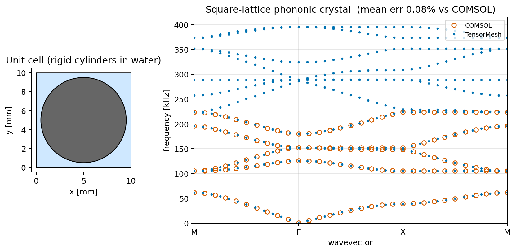
Fig. 43 Output of band_structure_square.py: the unit cell (left) and
the band structure along \(M\!-\!\Gamma\!-\!X\!-\!M\) (right),
TensorMesh bands as filled markers with the COMSOL reference as
open circles. The lowest band goes to zero at \(\Gamma\); band
gaps open between branches.
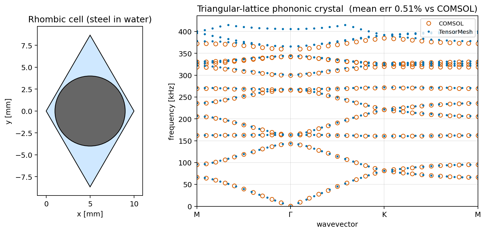
Fig. 44 Output of band_structure_triangular.py: penetrable steel
cylinders in water on a triangular lattice — a two-medium weighted
assembly on a non-orthogonal cell.
Transmission through a finite slab
transmission_slab.py leaves the infinite-crystal setting: a
normally-incident plane wave (\(p_0 = 1\) Pa) crosses a finite
slab of rigid cylinders, and the power transmission
\(T(f)=\langle|p|^2\rangle_{\mathrm{out}}/|p_0|^2\) is swept over
frequency:
mesh -> Laplace/Mass assembler -> (K - k^2 M - i k B) p = -2 i k p0 e_in
The first-order radiation term \(B\) and the incident load \(e_{\mathrm{in}}\) are hand-rolled boundary line integrals (no PML — this matches COMSOL’s first-order “Plane Wave Radiation” condition), and each frequency is one complex sparse solve. Inside the band gap the transmission drops to \(\sim 0\); in the pass bands it recovers with Fabry-Pérot ripples.
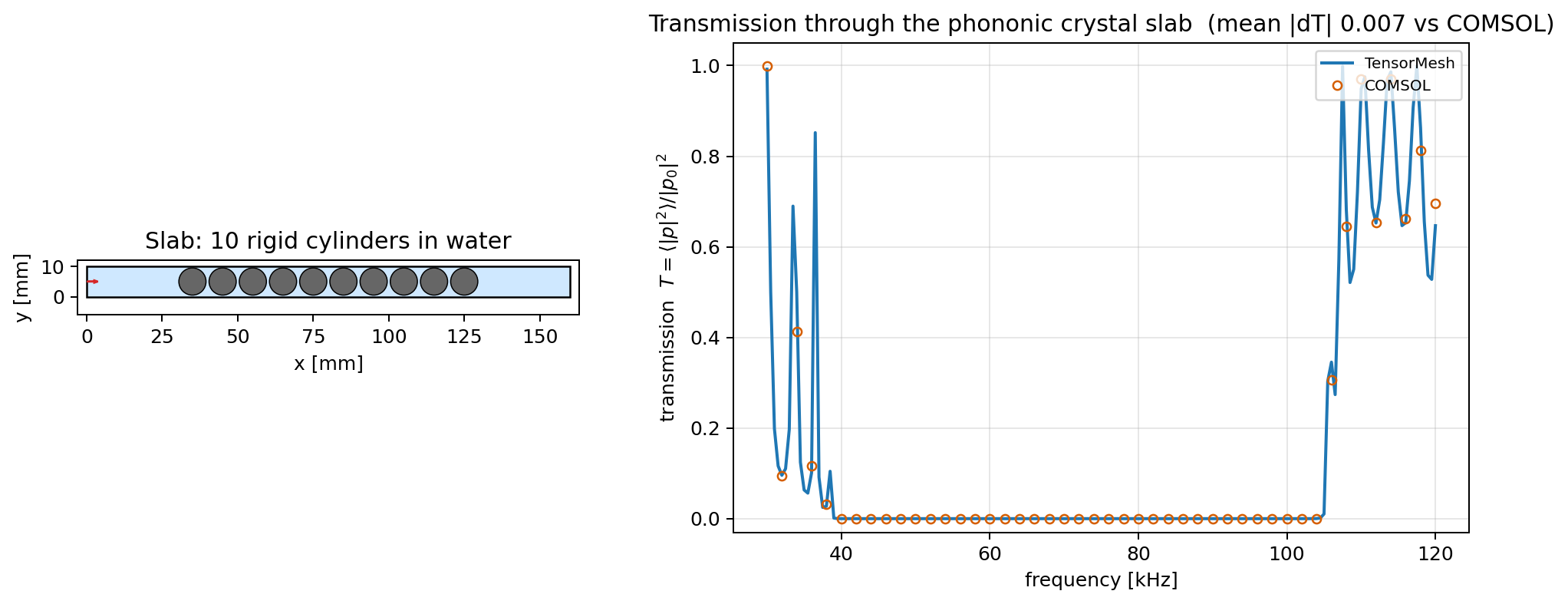
Fig. 45 Output of transmission_slab.py: the slab geometry (left) and
the transmission spectrum \(T(f)\) (right) with the COMSOL
reference overlaid — the band gap appears as the deep notch.
Validation against COMSOL
Each script overlays a COMSOL Pressure-Acoustics reference and prints
the relative error. The references are committed as small
comsol_reference_*.npz files next to the scripts, so the
comparison reproduces offline — no COMSOL needed:
Script |
Reference |
Agreement |
|---|---|---|
|
square \(M\!-\!\Gamma\!-\!X\!-\!M\), 31 k-points |
mean 0.08 %, p95 0.16 % |
|
triangular \(M\!-\!\Gamma\!-\!K\!-\!M\), 31 k-points |
mean 0.51 %, p95 1.45 % |
|
30-120 kHz, 46 frequencies |
mean \(|\Delta T|\) 0.007 |
Bands are compared k-point by k-point at COMSOL’s exact wavevectors (lowest 10 modes, nearest-frequency match); transmission by interpolating onto COMSOL’s frequency grid. If an npz is absent the script still runs and skips the overlay.
Running it
cd examples/wave/phononic_crystal_2d
python band_structure_square.py
python band_structure_triangular.py
python transmission_slab.py
Each script exposes a run_demo(...) returning diagnostics and a
main() with --no-plot, --output, and mesh-density /
band-count flags.
What’s next
Complex-Valued FEM — Helmholtz — the complex-valued Helmholtz machinery these examples build on.
Wave Equation — the time-domain wave equation.
BlochReducerin the API reference.