Open-Domain Wave (PML & Ports)
Frequency-domain wave problems on open domains need two ingredients beyond the plain complex Helmholtz assembly of Complex-Valued FEM — Helmholtz: a way to drive and absorb waves at a boundary (ports / first-order absorbing conditions), and a perfectly matched layer (PML) that soaks up outgoing radiation without reflection. Both shipped as small, composable operators:
robin_operator()/port_source()— the boundary matrix \(\int_\Gamma c\,N_iN_j\,\mathrm dS\) and incident load of a Robin / impedance / plane-wave-port condition, built onFacetBilinearAssembler(the bilinear counterpart ofFacetAssembler);cartesian_pml()— the stretched-coordinate PML tensor \(\mathbf\Lambda\) and mass scaling, consumed byAnisotropicLaplaceElementAssemblerandScaledMassElementAssembler.
Two worked examples in examples/wave/ exercise them — an acoustic
resonator driven through a port, and a photonic microdisk wrapped in a
PML frame.
Helmholtz resonator (acoustics, ports)
examples/wave/helmholtz_resonator/helmholtz_resonator.py solves a
2D duct with a necked side cavity — the textbook Helmholtz resonator —
driven by a plane-wave port at the inlet. All walls are sound-hard
(natural Neumann); the port both injects the incident wave and absorbs
the reflection:
In the weak form that is one boundary matrix and one boundary load on top of the usual stiffness/mass pair — the whole recipe is four lines:
from tensormesh import robin_operator, port_source

K = LaplaceElementAssembler.from_mesh(mesh)(points)
M = MassElementAssembler.from_mesh(mesh)(points)
B = robin_operator(mesh, inlet_mask)          # boundary mass on the port
e = port_source(mesh, inlet_mask)             # incident load

A = K - k**2 * M + 1j * k * B
p = A.solve(2j * k * p0 * e)                  # complex sparse solve
Sweeping the frequency and reading the input impedance \(Z(f) = p_{\text{avg}} / u_{\text{in}}\) at the inlet produces the resonance spectrum; the fundamental sits at 357 Hz with a cavity pressure gain of ~12x over the incident amplitude.
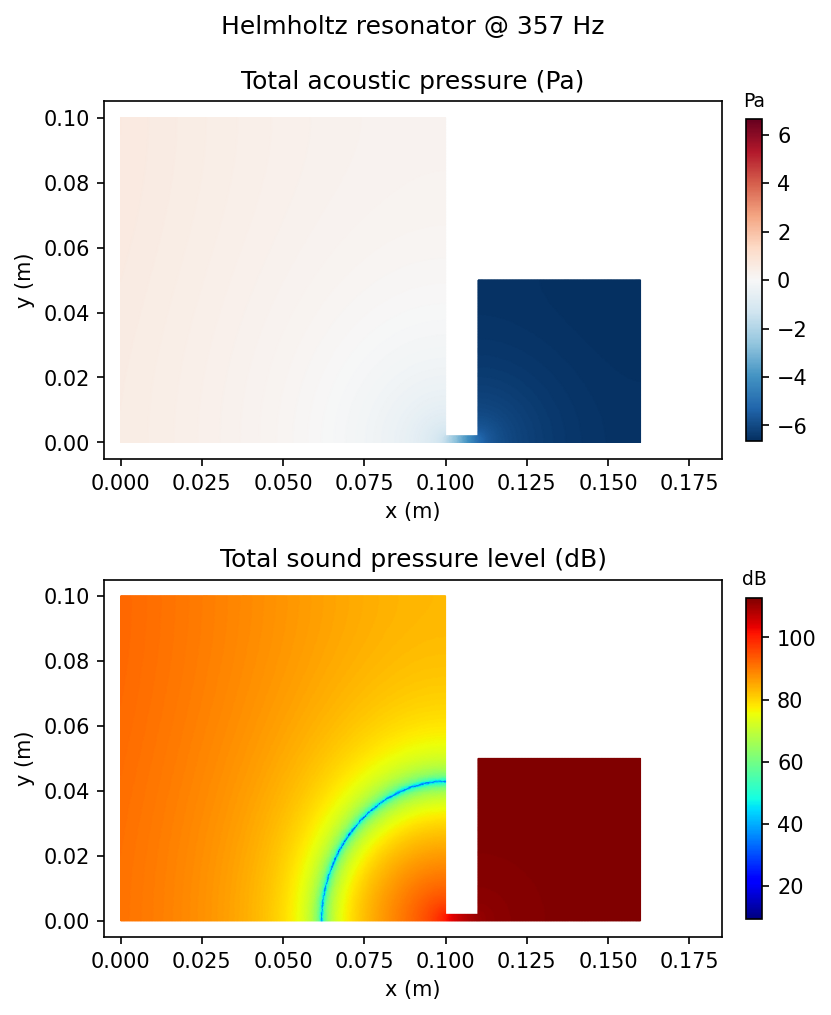
Fig. 46 The acoustic field at resonance: total pressure (top) and sound pressure level (bottom). The cavity rings at a nearly uniform high pressure while the duct stays quiet — the classic pressure-node line cuts across the neck.
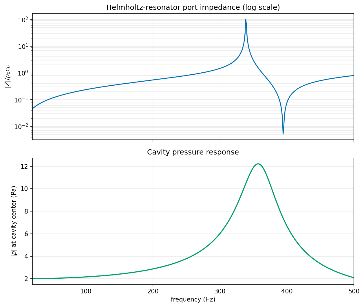
Fig. 47 Input impedance \(|Z|/Z_0\) over the sweep — the Helmholtz resonance and the duct harmonics appear as peaks, with anti-resonances between them.
Optical ring resonator (photonics, PML)
examples/wave/optical_ring_resonator/optical_ring_resonator.py is a
2D TM photonic solve: a silicon bus waveguide evanescently couples
light into a silicon microdisk (\(n = 3.48\)) in silica cladding
(\(n = 1.44\)), and a stretched-coordinate PML frame makes the
computational box behave as an open domain. The out-of-plane field
\(E_z\) obeys the PML-modified Helmholtz equation
with \(s_x = s_y = 1\) outside the layer. The reusable library path is three calls:
from tensormesh import cartesian_pml, AnisotropicLaplaceElementAssembler
from tensormesh.assemble import ScaledMassElementAssembler

Lam, s_prod = cartesian_pml(mesh.points, bounds=[(0, L), (0, L)], thickness=d)
K = AnisotropicLaplaceElementAssembler.from_mesh(mesh)(pts, point_data={"A": Lam})
M = ScaledMassElementAssembler.from_mesh(mesh)(pts, point_data={"c": eps_r * s_prod})
E = (K - k0**2 * M).solve(source)
(The example itself evaluates \(\varepsilon_r\) and the stretch per
quadrature point with an inline assembler for sharper Si/SiO₂
interfaces; the cartesian_pml path reproduces the same operator and
matches the 2D Hankel Green function to correlation 0.994.) A modal
soft source launches the guided bus mode directionally toward the disk.
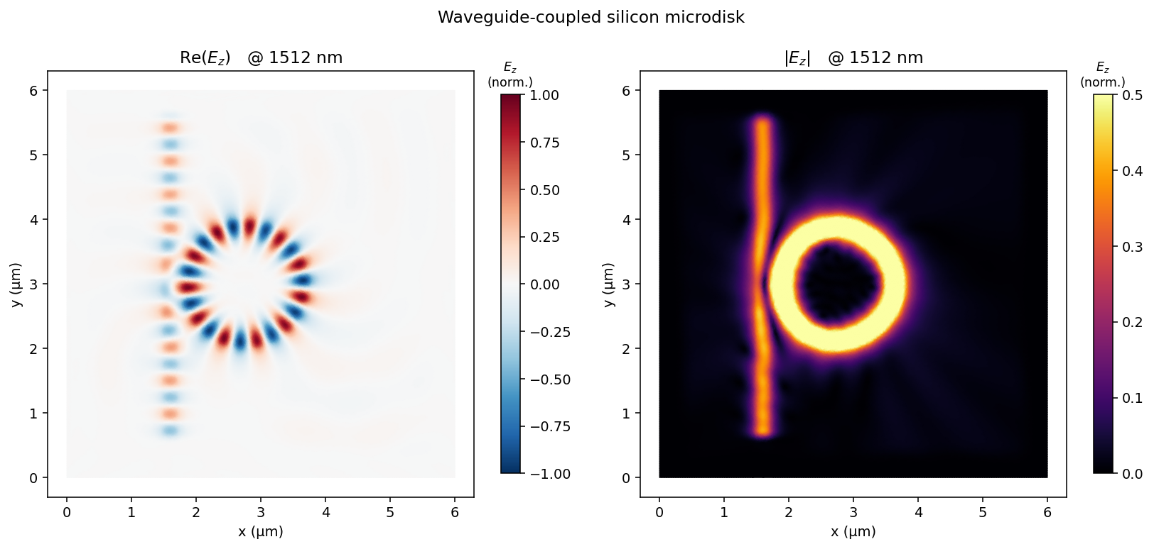
Fig. 48 On resonance the disk lights up in a whispering-gallery mode — a bright rim of azimuthal lobes (left: \(\mathrm{Re}\,E_z\), right: \(|E_z|\)), the bus waveguide visibly depleted past the coupling point, and the PML frame absorbing the radiated field.
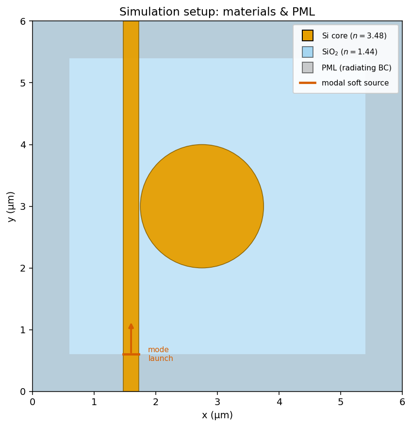
Fig. 49 The setup: materials, the two-plane directional launch, and the PML frame. Without the PML a hard box traps the radiation into a standing wave of ~8x the amplitude.
Running them
cd examples/wave/helmholtz_resonator && python helmholtz_resonator.py
cd examples/wave/optical_ring_resonator && python optical_ring_resonator.py
Both expose run_demo(...) returning diagnostics plus --no-plot
/ --output flags; the optical script also takes --lam0-nm,
--order and --mesh-h-nm (with P1 elements numerical dispersion
blue-shifts the physical 1.55 µm resonance to the default 1512 nm).
What’s next
Complex-Valued FEM — Helmholtz — the complex-valued assembly these operators build on.
Phononic Crystals (Bloch-Floquet) — the periodic counterpart (Bloch-Floquet boundary conditions instead of absorbing ones).
Modal Analysis — eigenmodes instead of driven responses.
FacetBilinearAssemblerin the API reference — write your own boundary bilinear forms (impedance, radiation damping, …).